DeepMind x UCL | Introduction To Reinforcement Learning (2015)

Watch the Lectures Here

Lecture 1: Introduction to Reinforcement Learning

Official Lecture Slides

RL is a fundamental science trying to understand the optimal way to make decisions.

A large part of the human brain / behavior is linked to a dopamine system (reward system), this neurotransmitter dopamine reflects exactly on one of the main algorithms we apply in RL.

About

Characteristic of Reinforcement Learning

Q. What makes reinforcement learning different from other Machine Learning Paradigms?

• There is no supervisor only a reward signal
  • No direct indication of correct / wrong action, instead it’s a trial and error paradigm.
• Feedback is delayed not instantaneous.
  • Initial decisions may reap rewards many steps later.
  • Example: A decision may instantaneously look good, and reap a positive reward for the next few steps, but then plunge into a large catastrophic negative reward!
• Time really matters (sequential, not i.i.d data)
  • Step after step, the agent gets to make a decision / pick an action and see how much reward it gets, accordingly optimizing those rewards to get the best possible outcome.
  • Unlike the classical supervised / unsupervised system we’re not talking about utilizing an IID dataset and learning from it, we’re facing a dynamic system: an agent moving through a world.
• Agent’s actions affect the subsequent data it receives
  • What the agent sees at the next step would be highly correlated to what it sees at the current step, furthermore as the agent gets to take action to influence its environment, in other words the agent is itself influencing it’s rewards (active learning process)!

Examples of Reinforcement Learning

• Fly stunt manoeuvres in a helicopter
• Defeat the world champion at Backgammon
• Manage an investment portfolio
• Control a power station
• Make a humanoid robot walk
• Play many different Atari games better than humans

The Reinforcement Learning Problem

Rewards

• A scalar / number feedback signal defined for every timestep t denoted by $R_t$, indicating how well the agent is doing at each timestep.
• The agent’s goal / job is to maximise the cummulative sum of these feedback signals / rewards.
• Reinforcement Learning is based on the reward hypothesis

Definition (Reward Hypothesis):

All goals can be described by the maximisation of expected cumulative reward.

Example Goal-Rewards

• Quickest to Target: Reward is set as -1 per timestep, hence the agent learns to take the least possible amount of steps.
• Fly Stunt manoeuvres in a trajectory:
  • +ve reward for following trajectory / large -ve reward for crashing
• Defeat the world champion at Backgammon: +/−ve reward for winning/losing a game
• Manage an investment portfolio: +ve reward for each $ in bank
• Control a power station:
  • +ve reward for producing power / large -ve reward for exceeding safety thresholds
• Make a humanoid robot walk:
  • +ve reward for forward motion / large -ve reward for falling over
• Play many different Atari games better than humans: +/−ve reward for increasing/decreasing score
• No intermediate rewards: We consider reward at the end of the episode to be the cummulative reward.

Sequential Decision Making

Although the examples we just discussed are all different from each other, we define a unifying framework for these by generalizing them to Sequential Decision Making Processes with the goal of selecting actions to maximize total future reward.

• Actions may have long term consequences, Ergo Reward may be delayed.
• This also means that at times the agent might have to sacrifice immediate reward to gain more long-term reward (non-greedy).

Examples:

• Blocking Opponent moves (might increase winning chances in future moves)
• Refuelling the helicopter (to avoid a crash in future)
• A financial investement (which would take a long period to mature)

Agent and Environment

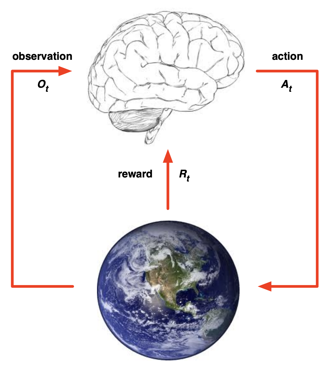
At each step $t$:

• The agent (brain):
  • Receives an observation $O_t$
  • Receives a reward $R_t$.
  • Takes an action $A_t$ based off of the information that it’s receiving from the world (observation $O_{t}$) and the reward signal it’s getting ($R_{t}$).
• The environment:
  • Receives an action $A_t$
  • Emits observation $O_{t+1}$
  • Emits scalar reward $R_{t+1}$
• $t$ increments at env step.

Thus, the trial and error loop that we define for Reinforcement Learning is basically a time series of observations, rewards and actions, which in turn defines the experience of an agent (which is the data we then use for reinforcement learning).

History & State

This stream of experience which comes in, i.e. the sequence of observations (all observable variables up till time t / incoming sensorimotor stream of the agent), actions & rewards is called history, and is denoted as:

\[H_t = O_1, R_1, A_1 \cdots, A_{t-1}, O_t, R_t\]

What happens next, then depends on this history:

• The agent selects an action
• The environment signals a reward and emits an observation

The history in itself however is not useful specially for agents which have long lives, as with increased time their processing speed would linearly reduce, real time interactions would become impossible. To resolve this, we instead talk about something called state, which is like a summary of the information which determines what happens next.

Formally, state is defined as a function of the history:

\[S_t = f(H_t)\]

Definitions of State

Environment State

• The information that’s used within the environment to decide what happens next, i.e. the environment’s private representation: $S_t^e$. In other words whatever data the environment uses to pick the next observation/reward.
• This state is not usually visible to the agent.

Hence, the environment state is more of a formalism, which helps us build the algorithms for our agent. Even if the environment state is visible, it might not directly contain relevant information for the agent to make good decisions.

Agent State

The agent state $S_t^a$ is a set of numbers that capture exactly what’s happened to the agent so far, summarize what’s gone on, what it’s seen so far and use those numbers to basically pick the next action. How we choose to process those observations and what to remember and what to throw away builds this state’s representation. It can be any function of the history:

\[S_t^a = f(H_t)\]

This is the information (agent state) used by RL algorithms.

Information / Markov State

An information state (a.k.a Markov state) contains all useful information of the history.

Definition (Markov State):

A state $S_t$ is markov if and only if:

\[\color{pink}\mathbb{P} [S_{t+1} | S_t] = \mathbb{P} [S_{t+1} | S_1, \cdots S_t]\]

in other words, you could throw away all previous states, as the current state in itself gets the same characterization (is a sufficient statistic) of the future.

• The future is independent of the past, given the present:

\[H_{1:t} \rightarrow S_t \rightarrow H_{t+1:\infty}\]

• The environment state $S_t^e$ is Markov.
• The history $H_t$ is also Markov (although inefficient). Hence it’s always possible to have a markov state, the question in practice is just how do we find that useful/efficient representation.

Rat Example

Consider the following classic, scientist-rat experiment scenario, say the rat observes these two sequences / experiences:

Next, in the current sequence, the rat observes the following sequence of states:

The expected next state by the rat, then depends on it’s representation of the state! For example:

• If the rat’s state depends on the sequence of last 3 observed states, then the rat expects to be zapped!
• If the rat’s state depends on the count of lever / light & bell, then it expects cheese!
• If the rat’s state depends on complete sequence, that it doesn’t know what to expect (not enough data)

Fully Observable Environments

In this specific scenario, the agent is able to directly observe the environment state:

\[O_t = S_t^a = S_t^e\]

• Agent State = Environment State = Information State
• Formally, this is called Markov Decision Process (MDP) (will be studied in the next lecture and the majority of this series).

Partially Observable Environments

In this specific scenario, the agent indirectly observes the environment:

• Examples:
  • A robot with a camera stream trying to figure out where it is in the world.
  • A trading agent only observing current prices
  • A poker playing agent only observing public cards

\[\texttt{Agent State} \neq \texttt{Environment State}\]

• Formally, this is called partially observable Markov Decision Process (POMDP).
• Agent must construct its own state representation in this case $S_t^a$, ex:
  • Complete history: $S_t^a = H_t$
  • Beliefs of Environment State: \(S_t^a = (\mathbb{P}[S_t^e = s^1], \cdots, \mathbb{P}[S_t^e = s^n])\)
  • Recurrent Neural Network: \(S_t^a = \sigma(W_s \cdot S_{t-1}^a + W_o \cdot O_t)\)

Inside an RL Agent

An RL agent may include one or more of these components (not exhaustive ofcourse!):

• Policy: agent’s behaviour function (how the agent decides what action to take when in a given state)
• Value function: how good is each state and/or action (how much reward do we expect if we take an action from a given state). In other words, estimating how well we are doing in a particular situation.
• Model: agent’s representation of the environment (how the agent thinks the environment works)

Policy

A policy is the agent’s behavior, it is a map from state to action, which may or may not be deterministic:

• Deterministic: $\pi(s) = a$
• Stochastic: $\pi(a \mid s) = \mathbb{P} [A=a \mid S=s]$

Value Function

The value function is a prediction of expected future reward, used to evaluate goodness/baddness of states, hence helping with action choice. Written as:

\[v_\pi(S) = \mathbb{E}_\pi[R_t + \gamma \cdot R_{t+1} + \gamma^2 \cdot R_{t+2} \cdots \mid s = S]\]

The behavior that maximizes this value, is the one that correctly trades off agent’s risk so as to get the maximum amount of reward going into the future. (Notice that the value function depends on the policy chosen $\pi$, here $\gamma \in [0,1]$ is the discount factor that determines how much we value future rewards vs immediate rewards)

Example: DQN Value Function in Atari (1:02:12 - 1:04:36)

Model

A model is basically not the environment itself but an estimate of what the environment might do. Hence, the agent tries and learns the behavior of the environment and then uses that model of the environment to help make a plan to help figure out what to do next. Generally, this model has two parts:

• Transitions: $\mathcal{P}$ predicts the next state (i.e. dynamics)
  • \[\mathcal{P}_{ss'}^{a} = \mathbb{P}[S' = s' \mid S = s, A = a]\]
• Rewards: $\mathcal{R}$ predicts the next (immediate) reward, e.g.
  • \[\mathcal{R}_{s}^{a} = \mathbb{E}[R \mid S = s, A = a]\]

It’s however not always required / necessary to build the environment’s model, in fact most of the lectures in this series will focus on model free methods instead.

Maze Example

In the above maze example, consider the following environment dynamics:

• Reward: -1 per time-step
• Actions: N E S W

• States: Agent’s location

• Fig. A represents the layout of the maze
• Fig. B represents the optimal deterministic policy mapping for each state,
• Fig. C represents value $v_\pi(s)$ for each state $s$
• Fig. D represents the agent’s internal environment model, after it traverses a path (might be imperfect):
  • The grid layout represents transition model $\mathcal{P}_{ss’}^{a}$
  • The numbers in each model state represent immediate reward $\mathcal{R}_{s}^{a}$ for each state $s$ (same for all $a$)

Categorizing RL Agents

• Taxonomy 1:
  • Value Based
    • No Policy (implicit) - Optimal Actions can be read out greedily based on value function
    • Value Function
  • Policy Based
    • Policy
    • No Value Function
  • Actor Critic
    • Policy
    • Value Function
• Taxonomy 2:
  • Model Free
    • Policy and/or value function
    • No Model
  • Model Based
    • Policy and/or value function
    • Model

Problems within Reinforcement Learning

Learning and Planning

Two fundamental problems in sequential decision making

• Reinforcement Learning:
  • The environment is initially unknown
  • The agent interacts with the environment
  • The agent improves its policy
  • Example (Atari): Learn to play a game from itneractive-gameplay by picking actions on joystick and observing pixels and scores.
• Planning:
  • A model of the environment is known
  • The agent performs computations with its model (without any external interaction)
  • The agent improves its policy
  • a.k.a. deliberation, reasoning, introspection, pondering, thought, search
  • Example (Atari): A queryable emulator ready at hand, which responds back with the next state and score based on current state and action (rules of the game are known). Using this model to plan ahead and find the optimal policy (ex: Tree Search).

Exploration and Exploitation

Reinforcement learning is like trial-and-error learning, we expect the agent to discover a good policy from its experiences of the environment, without losing too much reward along the way.

• Exploration finds more information about the environment, by possibly ignoring existing best-known reward policy
• Exploitation exploits known information to maximise reward
• It is usually important to explore as well as exploit

Examples:

• Restaurant Selection
  • Exploitation Go to your favourite restaurant
  • Exploration Try a new restaurant
• Online Banner Advertisements
  • Exploitation Show the most successful advert
  • Exploration Show a different advert

Prediction and Control

• Prediction: How well will the agent do if it follows a given policy. (value function prediction)
• Control: Finding the optimal policy to get the most reward
• In RL we typically need to solve the Prediction problem in order to solve the Control Problem, i.e. we evaluate all of our policies to figure out the best.

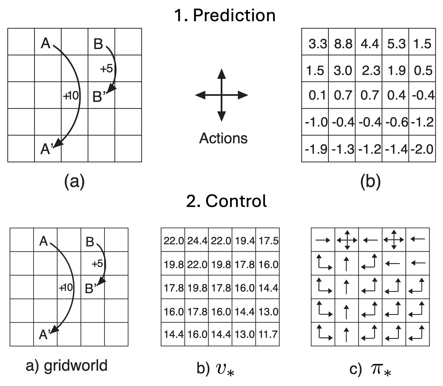
Example: Going back to our grid world with a -1 reward, we can possibly ask the following questions:

• Prediction: If we choose to randomly move across the grid, what’s our expected reward from a given state?
• Control: What’s the optimal behavior on the grid if I am in a given state? What’s the value function if I follow the optimal behavior?

Lecture 2: Markov Decision Process

Official Lecture Slides

Markov Processes / Chain

Introduction

Introduction to MDPs

Markov Decision Processes are a formal definition of the environment that the agent interacts with, applying only to the cases where the environment is fully observable.

In other words, the current state of the environment given to the agent completely characterizes this process (the way in which the environment unfolds depends on it). Almost all RL Problems an be formalized as MDPs, examples:

• Optimal control primarily deals with continuous MDPs
• Partially observable problems can be converted into MDPs
• Bandits are MDPs with one state (an agent is given a choice of actions, it chooses one.)

Markov Process

Markov Property

(already covered in Lecture 1, click on the shortcut above to refresh the concept!)

State Transition Matrix

Given a markov state $s$ and a successor state $s’$, the *state transition probability is defined by:

\[\mathcal{P}_{ss'} = \mathbb{P}[S_{t+1} = s' \mid S_t = s]\]

The state transition matrix $\mathcal{P}$, then defines transition probabilities from all states $s$ to all successor states $s’$.

\[\mathcal{P} = \text{from } \overset{\text{to}}{ \begin{bmatrix} \mathcal{P}_{11} & \dots & \mathcal{P}_{1n} \\ \vdots & \ddots & \vdots \\ \mathcal{P}_{n1} & \dots & \mathcal{P}_{nn} \end{bmatrix} }\]

Where, by the law of probability, each row sums to 1.

Markov Process / Chain

A Markov process is a memoryless random process, i.e. a sequence of random states $S_1, S_2, \cdots$ with the Markov property.

Definition (Markov Process):

A Markov Process (or Markov Chain) is a tuple $\langle\textcolor{pink}{\mathbfcal{S}, \mathbfcal{P}}\rangle$, where:

• $\color{pink}\mathcal{S}$ is a (finite) set of states

• $\color{pink}\mathcal{P}$ is a state transition probability matrix,

  \[\color{pink}\mathcal{P}_{ss'} = \mathbb{P}[S_{t+1} = s' \mid S_t = s]\]

Example: Student Markov Chain

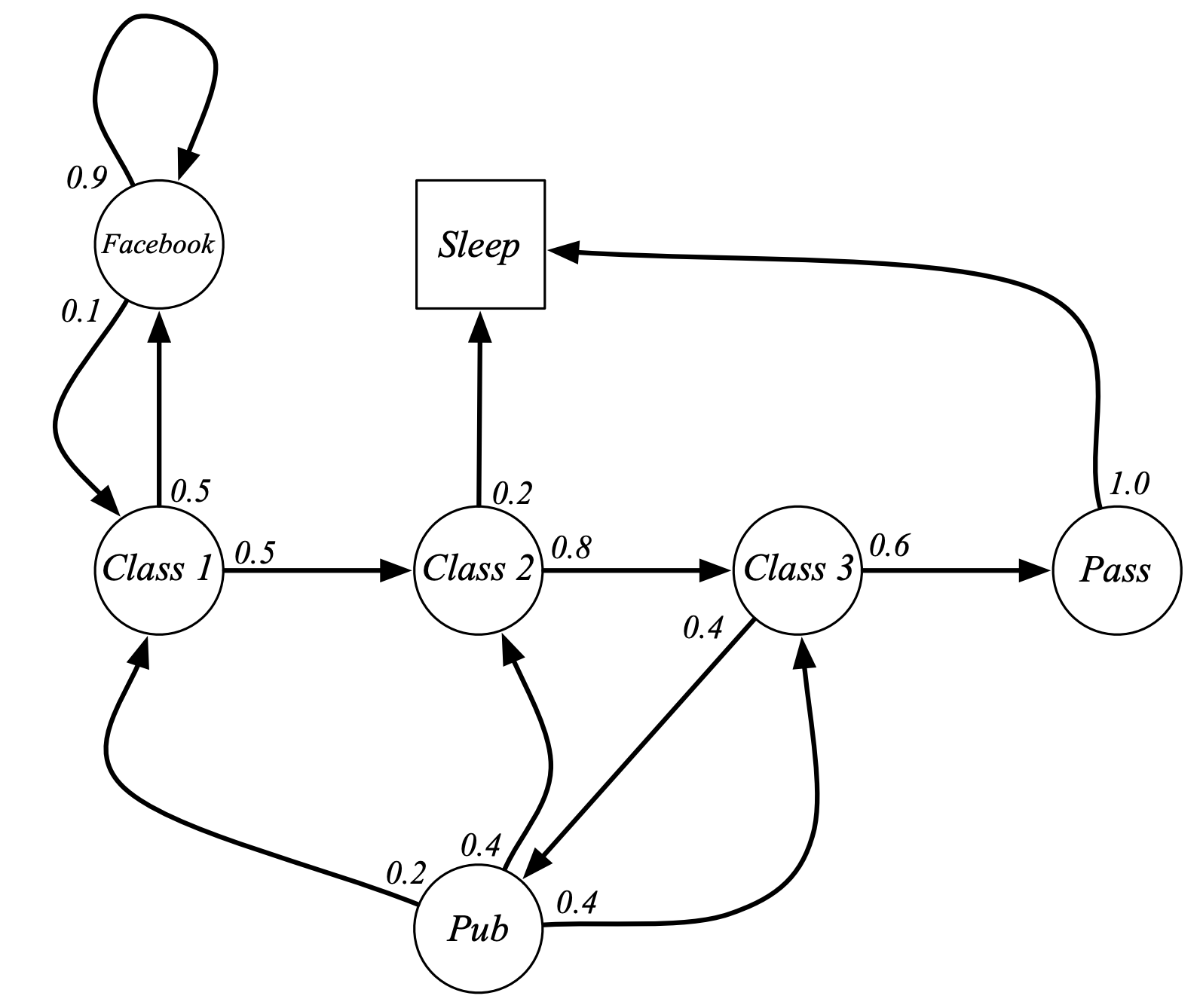
Notice that, “Sleep” is a terminal state which indefinitely keeps looping back to itself. Based on the above example chain, we can draw out sample episodes, starting from say $S_1 = C_1$:

• $C1, C2, C3, Pass, Sleep$
• $C1, FB, FB, C1, C2, Sleep$
• $C1, C2, C3, Pub, C2, C3, Pass, Sleep$
• $C1, FB, FB, C1, C2, C3, Pub, C1, FB, FB, FB, C1, C2, C3, Pub, C2, Sleep$

The above episodes are Random sequences that are drawn from a probability distribution over sequences of states and the fact it has the markov property means that it can be described by one of these diagrams. It can be described by saying from any state there’s some probability of transitioning to any other state.

\[\mathcal{P} = \begin{array}{r} \begin{array}{ccccccc} \small{C1} & \small{C2} & \small{C3} & \small{Pass} & \small{Pub} & \small{FB} & \small{Sleep} \end{array} \\ \begin{array}{r} \small{C1} \\ \small{C2} \\ \small{C3} \\ \small{Pass} \\ \small{Pub} \\ \small{FB} \\ \small{Sleep} \end{array} \left[ \begin{array}{ccccccc} & 0.5 & & & & 0.5 & \\ & & 0.8 & & & & 0.2 \\ & & & 0.6 & 0.4 & & \\ & & & & & & 1.0 \\ 0.2 & 0.4 & 0.4 & & & & \\ 0.1 & & & & & 0.9 & \\ & & & & & & 1 \end{array} \right] \end{array}\]

The above state transition matrix, summarizes the transition probabilities of the defined chain.

Q. How do we deal with modifications of these probabilities over time? Ex: Say that the probability of revisiting facebook decreases over time.

Ans. So there’s two answers to that:

• One answer is that you can have non-stationary Markov process, later we’ll have mdp so non-stationary mdp, in that case what you can do is use the same kind of algorithms we use for the stationary case but incrementally adjust your solution algorithm to just kind of track the best solution you found so far
• The other answer is to say well the fact you’ve got non-stationary Dynamics just makes it a more complicated markup process. Imagining for this scenario, that there’s probabilities that depend on how long you’ve been in this state and so forth so now you can ugment this state you can have a more complicated Mark process that has like a counter that tells you how long you’ve been in this Facebook State and now you’ve basically got lots of different states depending on whether you’ve been in Facebook once or twice or three times, ergo you can have an infinite / continuous set of these.

All of these things are possible but they don’t change the fundamental structure from this being a markov process this is just a particular simple instantiation where we can see everything on one page but don’t let that mislead you into thinking that markov processes are necessarily small or simple, we will solve very very complex markov processes in the rest of the course. We’ll see how to solve you know mdps sometime some of them have $10^{170}$ States. So you know, these could be very large and complex beasts with a lot of structure to them.

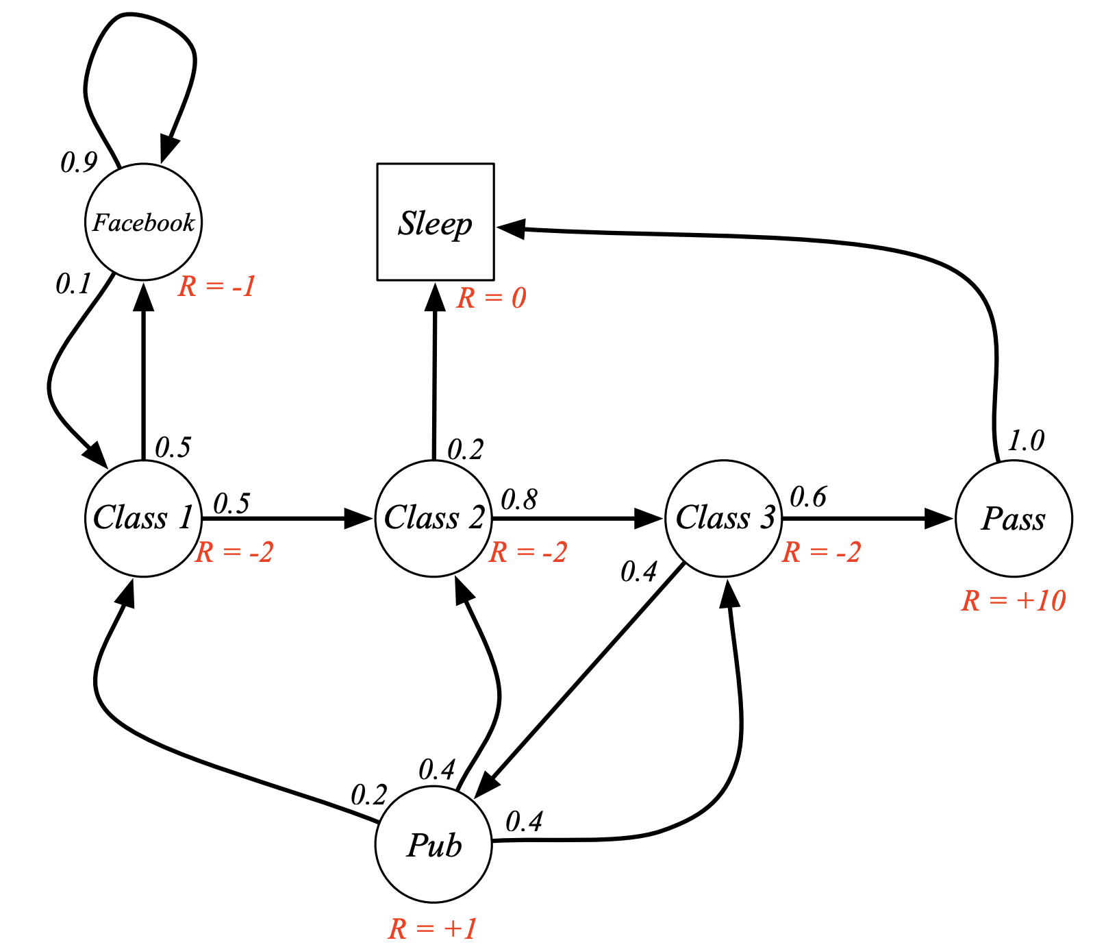
Markov Reward Processes (Markov Chain + Rewards)

Introduction

A Markov Reward Process is a Markov Chain with value judgements (saying how much reward will the agent have accumulated across some particular sequence that we sampled from a given Markov process).

Definition (Markov Reward Process):

A Markov Reward Process is a tuple $\langle\mathcal{S}, \mathcal{P}, \textcolor{pink}{\mathbfcal{R}, \boldsymbol\gamma}\rangle$, where:

• $\mathcal{S}$ is a (finite) set of states

• $\mathcal{P}$ is a state transition probability matrix,

  \[\mathcal{P}_{ss'} = \mathbb{P}[S_{t+1} = s' \mid S_t = s]\]
• $\textcolor{pink}{\mathbfcal{R}}$ is a reward function, $\mathcal{R_s} = \mathbb{E}[\mathcal{R}_{t+1} \mid \mathcal{S}_t = s]$
• $\textcolor{pink}{\boldsymbol\gamma}$ is a discount factor, $γ \in [0, 1]$

Example: Student Markov Reward Process

Return

Definition (Return):

For a given sample experience drawn from the chain, the return $\textcolor{pink}{\mathbf{G_t}}$ is defined as: \(\color{pink}G_t = R_{t+1} + \gamma \cdot R_{t+2} + \gamma^2 \cdot R_{t+3} \cdots = \sum_{k=1}^{\infty}\gamma^k\cdot R_{t+1+k}\)

The discount factor $\gamma$ (how much we care now for the rewards we get in the future) weighs immediate reward over delayed reward:

• $\gamma$ close to 0 leads to: myopic evaluation
• $\gamma$ close to 1 leads to: farisghted evaluation

Why Discount?

• It’s Mathematically convenient to discount rewards, avoids infinite returns in cyclic Markov processes too
• Uncertainty about the future may not be fully represented (i.e. we are uncertain about the accuracy of our model, and hence choose to trust later predicted rewards less)
• Animal/human behaviour shows preference for immediate reward (ex: financial rewards).

Although, It is sometimes possible to use undiscounted Markov reward processes (i.e. $\gamma=1$), e.g. if all sequences terminate.

With the average reward formulation, it’s possible even with infinite sequences to still deal with the undiscounted evaluation of markov processes processes and mdps. (Discussed in extend notes of this class)

Value Function

The value function $v(s)$ gives the long-term value of state s (i.e. the expected return if the agent starts an episode from state s). Definition (Value Function):

The state value function v(s) of an MRP is the expected return starting from state s:

\[v(s) = \mathbb{E}[G_t \mid S_t = s]\]

Example

Sample returns for Student MRP, Starting from $S_1 = C_1$ with $\gamma=\frac{1}{2}$: 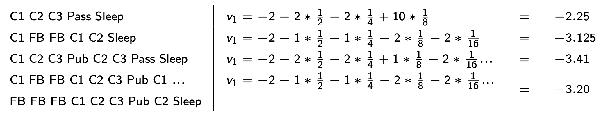(Although the selected episodes for which the returns are calculated are random, but the calculated values for these states individually (next figure) won’t be a random quantity, as it’s an expectation over these random quantities.)

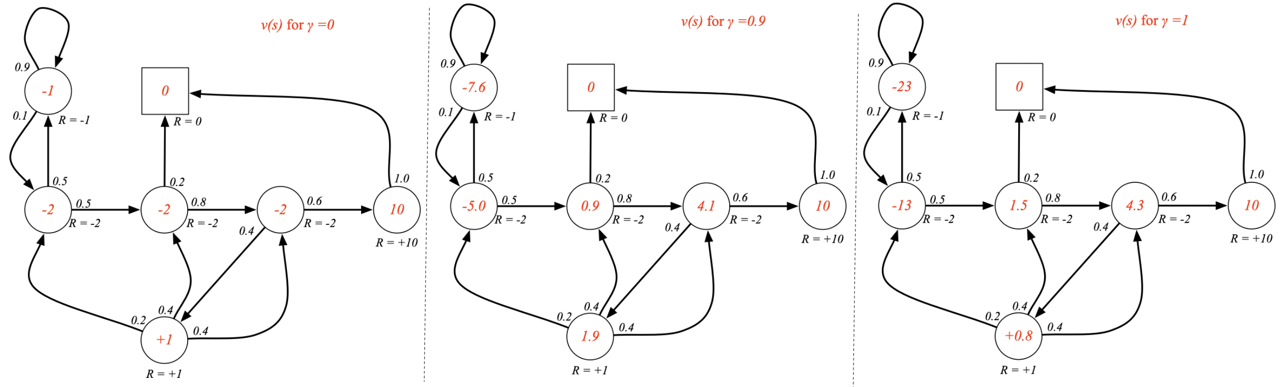
Bellman Equation for MRPs

The value function obeys a recursive decomposition consisting of the following two parts:

• immediate reward $R_{t+1}$
• Discounted value of the successor state: $\gamma \cdot G_{t+1}$

\[\begin{aligned} v(s) &= \mathbb{E}[G_t \mid S_t = s] \\ &= \mathbb{E}[R_{t+1} + \gamma \cdot R_{t+2} + \gamma^2 \cdot R_{t+3} + \cdots \mid S_t = s] \\ &= \mathbb{E}[R_{t+1} + \gamma \cdot (R_{t+2} + \gamma R_{t+3} + \dots) \mid S_t = s] \\ &= \mathbb{E}[R_{t+1} + \gamma G_{t+1} \mid S_t = s] \\ &= \mathbb{E}[R_{t+1} + \gamma \cdot v(S_{t+1}) \mid S_t = s] \end{aligned}\]

(The transition from the second last to last step comes from the law of expected iterations, which states that the overall expected value of a random variable $X$, $\mathbb{E}[X]$, can be found by first taking the conditional expectation of $X$ given another variable $Y$, $\mathbb{E}[X\mid Y]$, and then averaging these conditional expectations over all possible values of $Y$. Mathematically, this is expressed as $E[X]=E[E[X\mid Y]]$)

We do one-step lookaheads, by moving one step ahead from current state, take an average of all possible outcomes (with transition probabilities) together, which gives us the value function at the current step.

\[v(s) = \mathcal{R}_s + \gamma\sum_{s' \in S} \mathcal{P}_{ss'}\cdot v(s')\]

Here is a backup diagram (what’s a backup diagram?) of this process: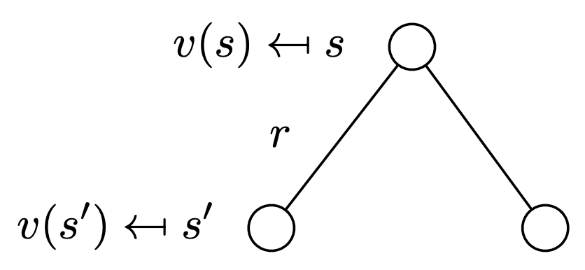

Student MRP Example

The below figure shows equivalence of the value at a given state to the immediate reward and a discounted (just 1 in this case) average of lookaheads for a converged value function for the Student MRP with a $\gamma$ factor of 1: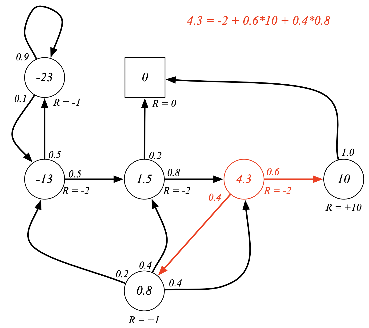

Matrix Representation

\(\left[\begin{matrix}v(1)\\\vdots\\v(n)\end{matrix}\right] = \left[\begin{matrix}\mathcal{R}_1\\\vdots\\\mathcal{R}_n\end{matrix}\right] + \gamma \begin{bmatrix} \mathcal{P}_{11} & \dots & \mathcal{P}_{1n} \\ \vdots & \ddots & \vdots \\ \mathcal{P}_{n1} & \dots & \mathcal{P}_{nn} \end{bmatrix} \left[\begin{matrix}v(1)\\\vdots\\v(n)\end{matrix}\right]\)

Solving the Bellman Equation

As can be seen, the bellman equation is linear and can be solved directly:

\[\begin{aligned} v &= \mathcal{R} + \gamma \cdot \mathcal{P}v \\ &= (1 - \gamma \cdot \mathcal{P})^{-1} \mathcal{R} \\ \end{aligned}\]

However, the time-complexity for this borders around $n^3$ (due to the inverse calculation), and hence it practically only applies to small MRPs. For larger MRPs, we go for other iterative solutions such as:

• Dynamic programming
• Monte-Carlo evaluation
• Temporal-Difference learning

Another point to note is that this nice linear property goes away, once we move to MDPs, where instead of evaluating Rewards, we are looking for max possible rewards for each state, which makes the above equation more complex.

Markov Decision Processes (Markov Chain + Rewards + Actions)

Introduction

A Markov decision process (MDP) is a Markov reward process with decisions. It is an environment in which all states are Markov.

Definition (Markov Decision Process):

A Markov Decision Process is a tuple $\langle\mathcal{S}, \textcolor{pink}{\mathbfcal{A}}, \mathcal{P}, \mathbfcal{R}, \boldsymbol\gamma\rangle$, where:

• $\mathcal{S}$ is a (finite) set of states
• $\textcolor{pink}{\mathbfcal{A}}$ is a (finite) set of Actions

• $\mathcal{P}$ is a state transition probability matrix,

  \(\mathcal{P}_{ss'}^\textcolor{pink}{a} = \mathbb{P}[S_{t+1} = s' \mid S_t = s, \textcolor{pink}{A_t = a}]\) (Notice that the transition probability from one state to another may depend on the selected action too now)

• $\mathbfcal{R}$ is a reward function, \(\mathcal{R_s^\textcolor{pink}{a}} = \mathbb{E}[\mathcal{R}_{t+1} \mid S_t = s,\textcolor{pink}{A_t = a}]\) (Notice that the reward may depend on the selected action too now)
• $\boldsymbol\gamma$ is a discount factor, $γ \in [0, 1]$

Example: Student Markov Decision Process

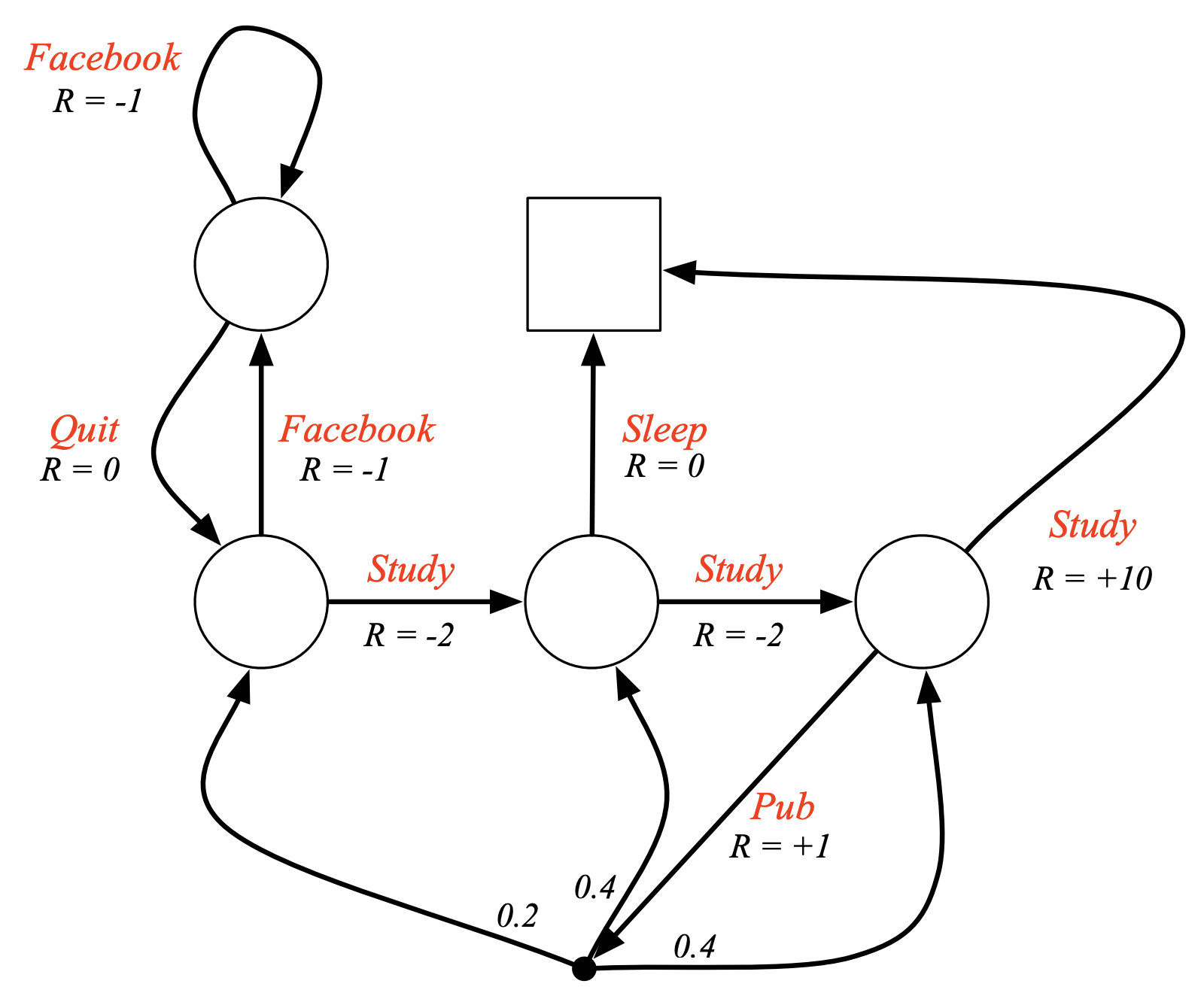
Notice now that, there are no probabilities attached to probable transitions from one state to the other, that is we’re free to move about the states (take decisions / make choices), each transition now has a dedicated reward.

Notice that, post taking the action the agent doesn’t always deterministically land on a state, the environment may influence which state the agent lands in. As an example consider that the agent lands in the class 3 node and chooses the “Pub” action, thereby gaining a reward of $-2$, next it depends on the environment to which node it wishes to push the agent to, in the current scenario, the environment pushes the agent to class 1 with probability 0.2 & classes 2 & 3 with probability 0.4 each.

There’s a lot more control that the agent can exert now over its path through this mdp. This is the reality for an agent and the goal / the game we’ll be playing now is to try and find the best path through our decision making process that maximizes the sum of rewards that the agent gets.

Policies

Definition (Policy):

A policy $\pi$ is a distribution over actions given states,

\[\pi(a \mid s) = \mathbb{P}\left[A_t = a \mid S_t = s\right]\]

• A policy fully defines the behavior of the agent
• MDP policies depend only on the current state (not the history), in other words, policies are stationary: \(A_t = \pi(.|S_t), \forall t \gt 0\)
• It’s useful to make the policy stochastic because that allows us to do things like exploration (more on this later in the lectures)
• We can always recover a Markov Process or a Markov Reward Process from a Markov Decision Process. Given an MDP \(\mathcal{M} = \langle \mathcal{S}, \mathcal{A}, \mathcal{P}, \mathcal{R}, \gamma \rangle\) and a policy $\pi$, we can define a:
  • MP from a MDP as $\Rightarrow$ $\langle \mathcal{S}, \mathcal{P^\pi} \rangle$ for a state sequence: $S_1, S_2, S_3, \cdots$
  • MRP from a MDP as $\Rightarrow$ $\langle \mathcal{S}, \mathcal{P^\pi}, \mathcal{R^\pi}, \gamma \rangle$ for a state-reward sequence $S_1, R_2, S_2, \cdots$
  • Where:
    • $\mathcal{P_{ss’}^\pi} = \sum_{a \in A}\pi(a\mid s) \mathcal{P_{ss’}^a}$
    • $\mathcal{R_{s}^\pi} = \sum_{a \in A}\pi(a\mid s) \mathcal{R_{s}^a}$

Value Function

Definition (Value Function):

The state-value function $v_{\pi}(s)$ of an MDP is the expected return starting from state $s$, and then following policy $\pi$

\[v_{\pi}(s) = \mathbb{E}_{\pi}\left[G_t \mid S_t = s\right]\]

Definition (Action-Value Function):

The action-value function $q_{\pi}(s,a)$ of an MDP is the expected return starting from state $s$, taking action $a$ and then following policy $\pi$

\[q_{\pi}(s,a) = \mathbb{E}_{\pi}\left[G_t \mid S_t = s, A_t = a\right]\]

Note that $\mathbb{E}_{\pi}$ indicates, expected value given that we’re sampling from the MDP while following policy $\pi$

Example: State-Value Function for Student MDP

Bellman Expectation Equation

The state-value function can again be decomposed into immediate reward plus discounted value of successor state:

\[v_{\pi}(s) = \mathbb{E}\left[R_{t+1} + \gamma\cdot v_{\pi}(S_{t+1}) \mid S_t = s\right]\]

Similarly for the action-value function:

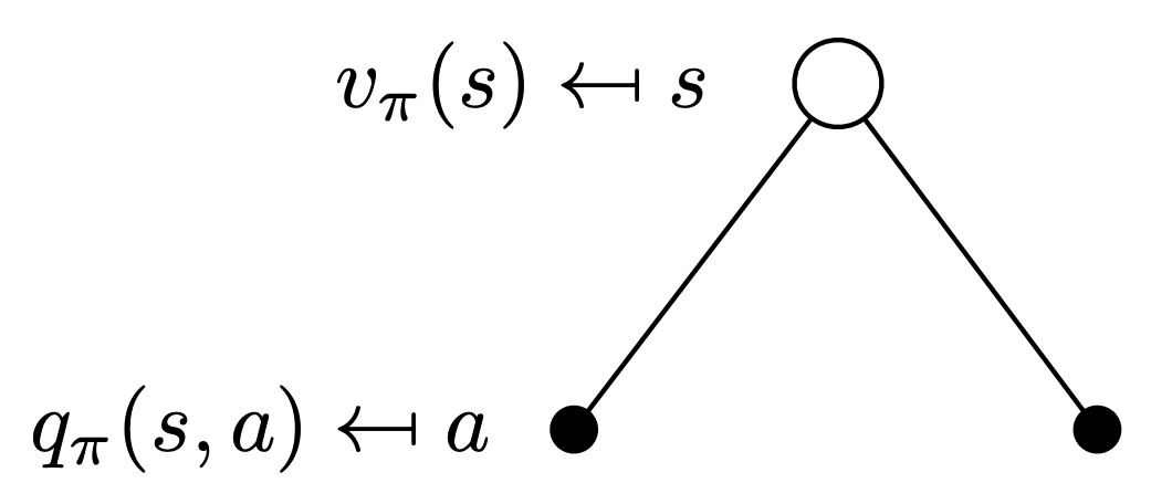
\[q_{\pi}(s, a) = \mathbb{E}\left[R_{t+1} + \gamma\cdot q_{\pi}(S_{t+1}, A_{t+1}) \mid S_t = s, A_t = a\right]\]

Now, consider the following backup diagram, which indicates the value function at a given state. From a given state, we choose actions, and when following a policy $\pi$, we choose these actions with a probability of $\pi(a\mid s)$. For each chosen action from a given state, we have an expected reward from there-on defined by the action value function: $q_{\pi}(s, a)$. Thus, we get:

\[v_{\pi}(s) = \sum\limits_{a \in \mathcal{A}}\pi(a\mid S) q_{\pi}(s, a)\]

Following the previous chain of thought, now consider the fact that we have chosen a given action from a state, which directly gives us the immediate reward. Next, depending on the stochasticity of the environment, we may now landup in one of the many probable states post taking an action, as we already know the probability of this is given by: $\mathcal{P_{ss’}^a}$. Hence, we can write the action-value function at a given action choice from a state as: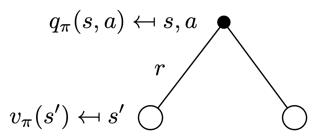

\[q_{\pi}(s, a) = R_{s}^a + \gamma \sum\limits_{s' \in \mathcal{S}}\mathcal{P_{ss'}^a} v_{\pi}(s')\]

Notice that, the expected reward coming from the second term is from next step and thus discounted.

Bellman Expectation Equation for $v_{\pi}(s)$

Combining the above 2 observations, we can now write a recursive relation for the state-value function as: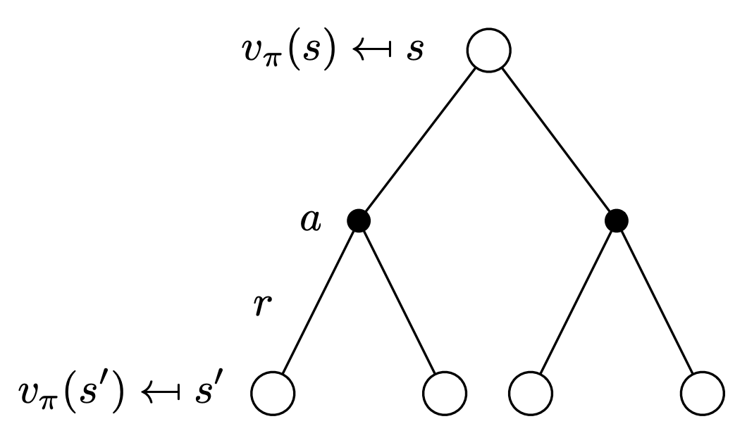

\[v_{\pi}(s) = \sum\limits_{a \in \mathcal{A}}\pi(a\mid S)(R_{s}^a + \gamma \sum\limits_{s' \in \mathcal{S}}\mathcal{P_{ss'}^a} v_{\pi}(s'))\]

Bellman Expectation Equation for $q_{\pi}(s,a)$

Similarly, we can now write a recursive relation for the action-value function as: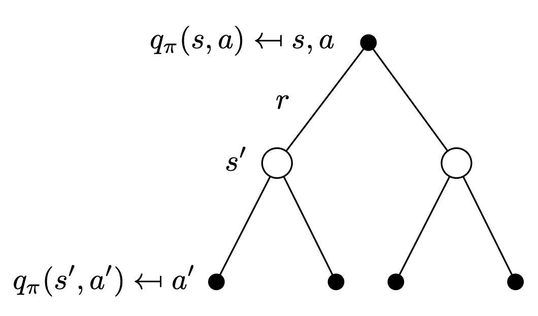

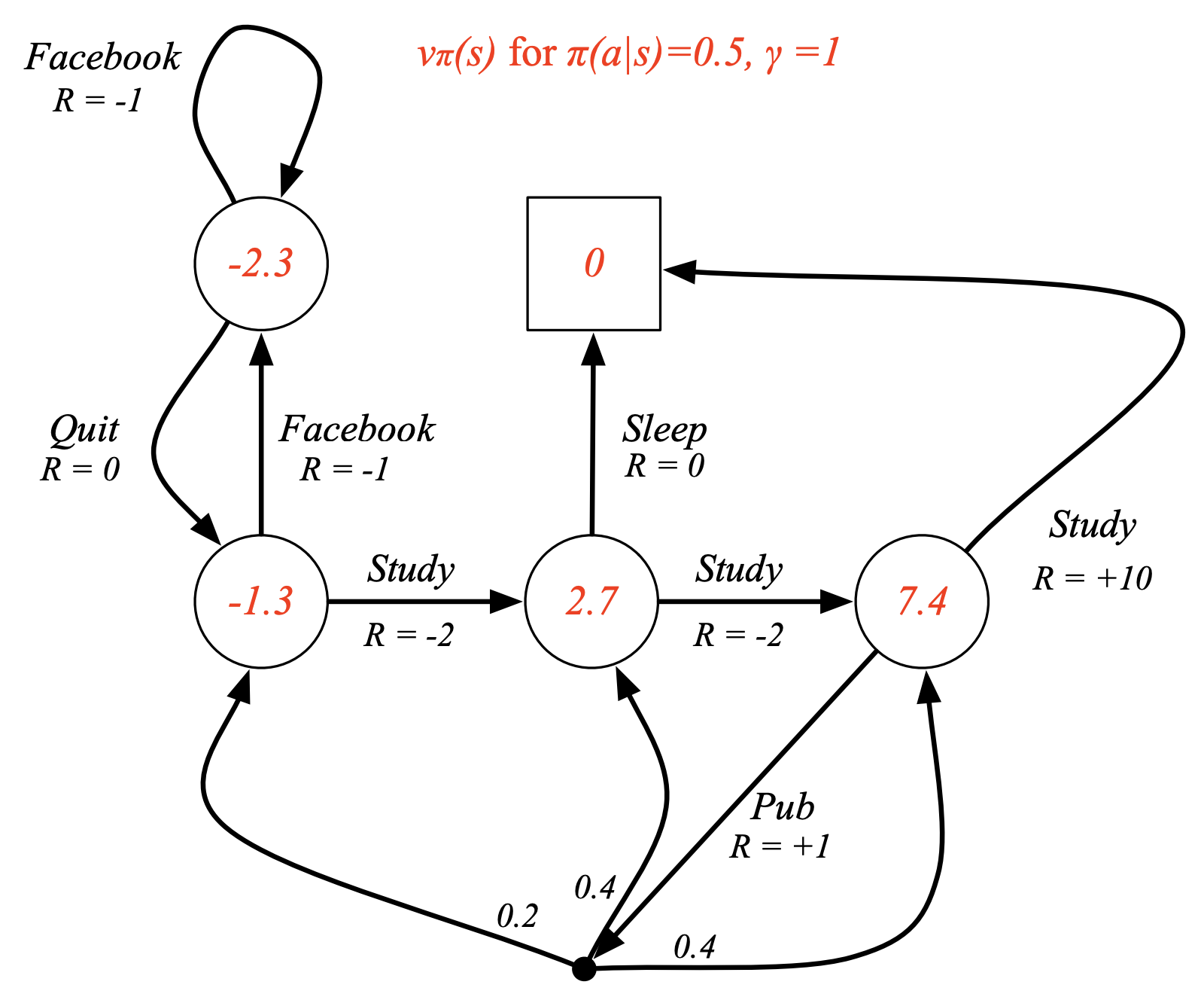
\[q_{\pi}(s, a) = R_{s}^a + \gamma \sum\limits_{s' \in \mathcal{S}}\mathcal{P_{ss'}^a}(\sum\limits_{a' \in \mathcal{A}}\pi(a'\mid s') q_{\pi}(s', a'))\]

Example: Bellman Expectation Equation for Student MDP

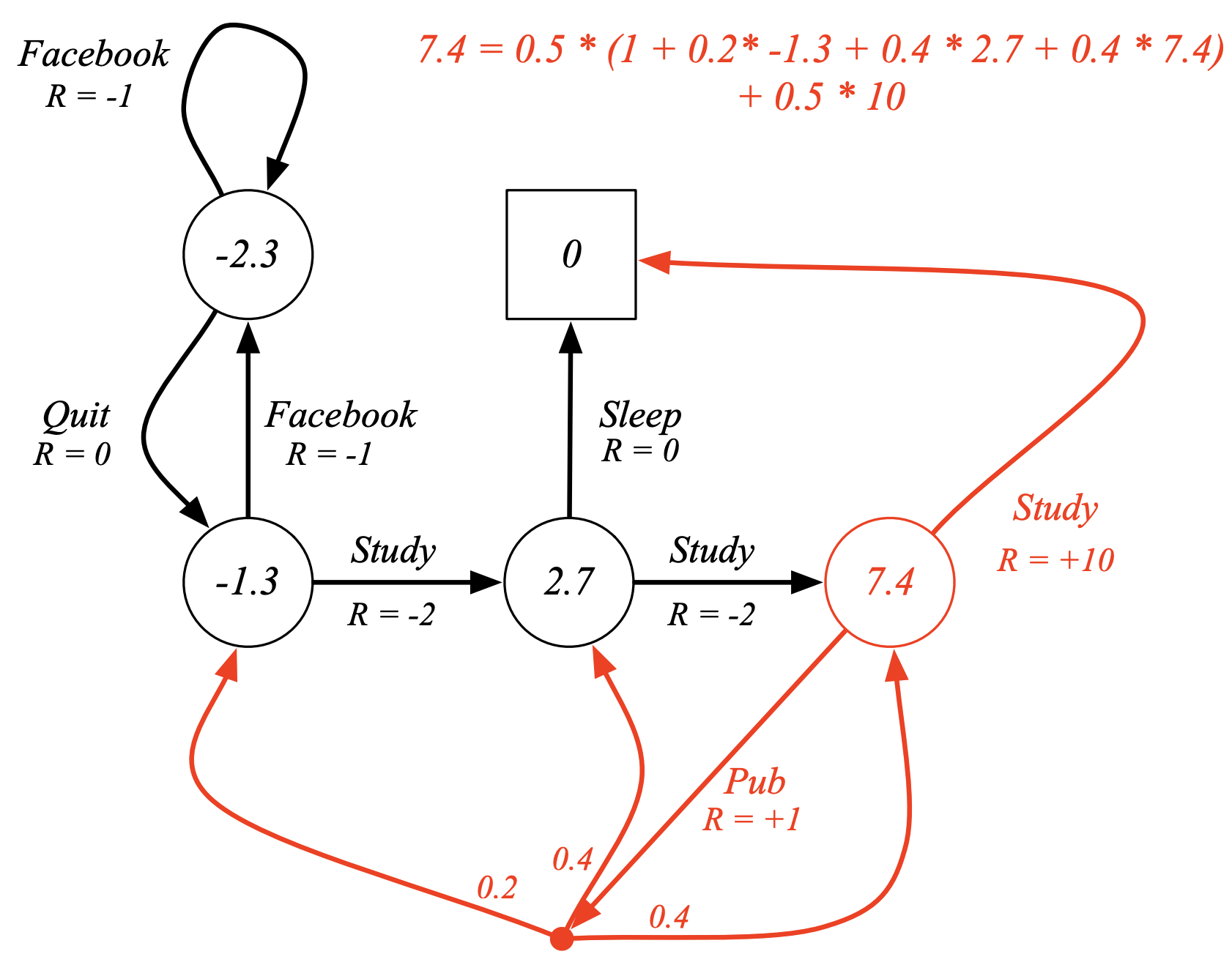
The above example, illustrates verification of the converged value for the state-value function at a given state (Class 3), such that $\pi(a \mid s) = 0.5$ & $\gamma = 1$.

Matrix Representation

Alternatively, we can represent the state-value function solution via matrix representation by converting our MDP to MRP, as discussed earlier here and here:

\[\begin{aligned} v_{\pi} &= \mathcal{R^{\pi}} + \gamma \cdot \mathcal{P^{\pi}}v_{\pi} \\ &= (1 - \gamma \cdot \mathcal{P^{\pi}})^{-1} \mathcal{R^{\pi}} \\ \end{aligned}\]

Optimal Value Function

Definition (Optimal Value Function):

The optimal state-value function $v_{*}(s)$ is the maximum value function over all policies:

\[v_{*}(s) = \underset{\pi}{\text{max}} \quad v_{\pi}(s)\]

The optimal action-value function $q_{*}(s, a)$ is the maximum action-value function over all policies

\[q_{*}(s, a) = \underset{\pi}{\text{max}} \quad q_{\pi}(s, a)\]

• The optimal value function specifies the best possible performance in the MDP.
• An MDP is solved, when we know the optimal value function.

To study in depth about conditions under which Markov Processes are well-defined refer to Dynamic Programming and Optimal Control (Volume II) by Dimitri P. Bertsekas.

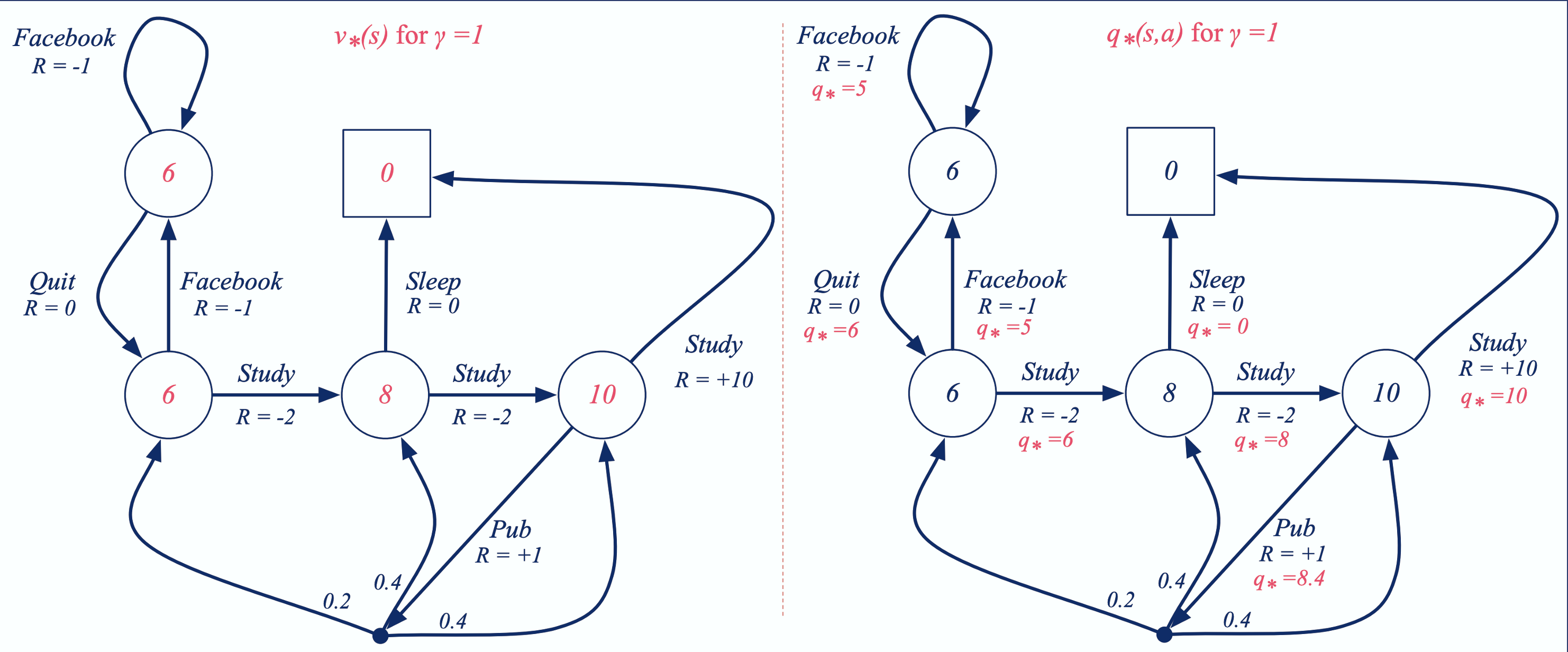
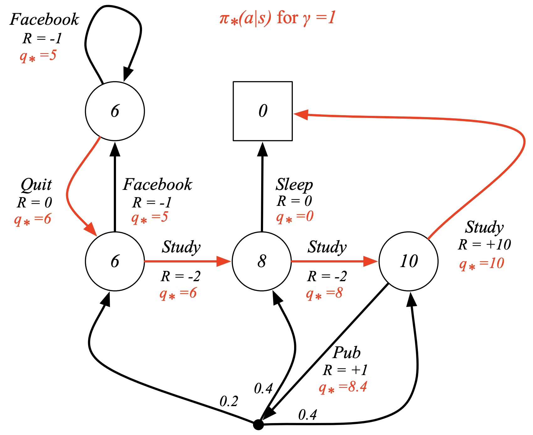
Example: Optimal Value Functions for Student MDP

Optimal Policy

We define a partial ordering over policies, by:

\[\pi \ge \pi^*\quad\text{if}\quad v_{\pi}(s) \ge v_{\pi^*}(s) \forall s\]

Theorem:

For any Markov Decision Process:

• There exists altleast one optimal policy \(\pi^{*}\) that is better than or equal to all other policies:

  \[\pi^* \ge \pi \forall \pi\]

• All optimal policies achieve the optimal value function:

  \[v_{\pi^*}(s) = v_{*}(s)\]

• All optimal policies achieve the optimal action-value function,

  \[q_{\pi^*}(s, a) = q_{*}(s, a)\]

Finding an Optimal Policy

An optimal policy can be found by maximising over $q_{*}(s,a)$:

\[\pi_{*}(a|s) = \begin{cases} 1, & \text{if } a = \underset{a \in A}{\text{argmax}} \ q_{*}(s,a) \\ 0, & \text{else } \\ \end{cases}\]

• There is always an optimal deterministic policy for any MDP
• If we know $q_{*}(s,a)$, we immediately have the optimal policy

Optimal Policy for student MDP

Bellman Optimality Equation

The optimal value functions are recursively related by the Bellman optimality equations:

• Consider the following backup diagram, which indicates the optimal state-value function at a given state (notice that unlike the expectation equation, we take the max and not weighted average!)

  

  \[v_*(s) = \underset{a \in A}{\text{max}} \ q_*(s, a)\]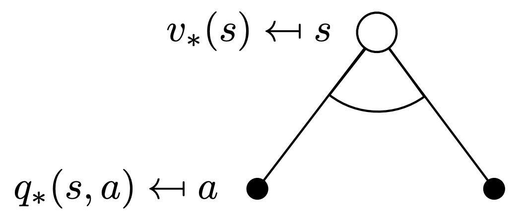

• Consider the following backup diagram, which indicates the optimal action-value function at a given state (we can’t take a max here, as the state transition probabilites are not in our control! they’re dependent on the environment)

  

  \[q_*(s, a) = \mathcal{R}_s^a + \sum_{s' \in \mathcal{S}} \mathcal{P_{ss'}^a} v_*(s')\]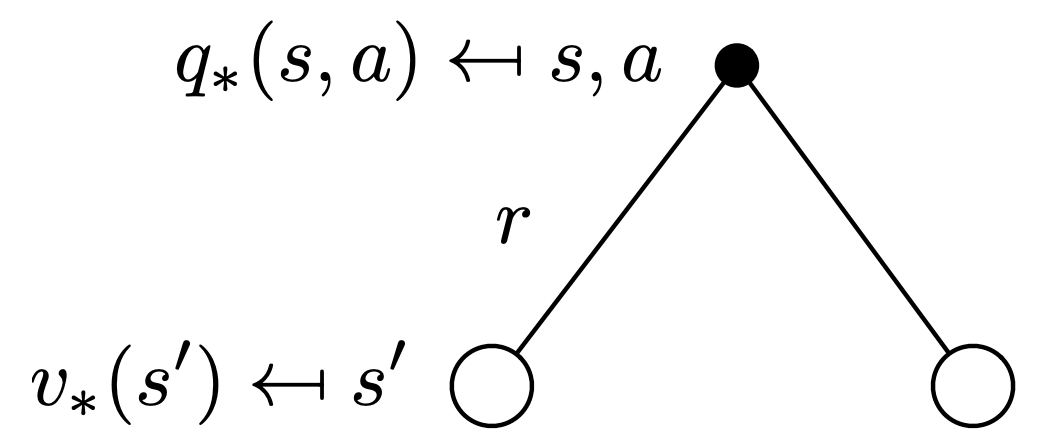

For $v_*$

Combining the above 2 observations, we can now write a recursive relation for the optimal state-value function as:

\[v_*(s) = \underset{a \in A}{\text{max}} \ (\mathcal{R}_s^a + \sum_{s' \in \mathcal{S}} \mathcal{P_{ss'}^a} v_*(s'))\]

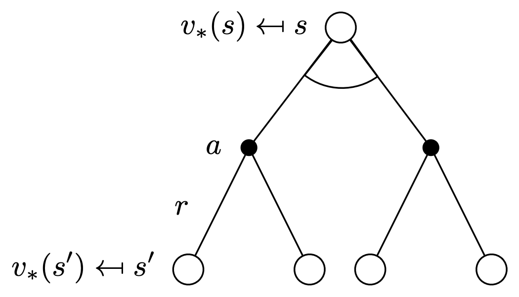
Here’s an example from the Student MDP, illustrating this relation: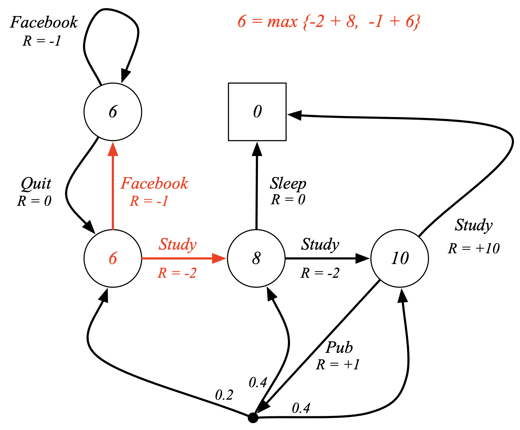

For $Q^*$

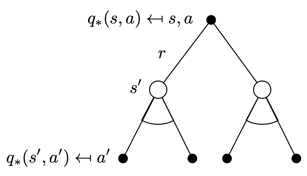
Similarly, we can now write a recursive relation for the optimal action-value function as:

\[q_*(s, a) = \mathcal{R}_s^a + \sum_{s' \in \mathcal{S}} \mathcal{P_{ss'}^a} \ \underset{a' \in A}{\text{max}} \ q_*(s', a')\]

Solving the Bellman Optimality Equation

• Bellman Optimality Equation is non-linear
• No closed form solution (in general)
• Many iterative solution methods
  • Value Iteration
  • Policy Iteration
  • Q-learning
  • Sarsa

FAQs

• Q1. How can uncertainty and model imperfection be handled in Markov Decision Processes (MDPs)?

  Ans. An MDP is only an approximate model of a real-world environment, so uncertainty is unavoidable. There are several ways to represent and manage this imperfection:

  1. Bayesian / Explicit Uncertainty Modeling
     • Maintain a posterior distribution over possible MDP dynamics.
     • Solve for a policy that is optimal across a distribution of MDPs, rather than a single one.
     • This approach is principled but computationally very expensive.
  2. Augmenting the State to Implicitly Encode Uncertainty
     • Incorporate uncertainty directly into the state representation.
     • For example, a state may include:
       • The agent’s physical configuration, and
       • Beliefs about the environment’s dynamics, or
       • The history of observations so far.
     • This avoids explicit reasoning over all uncertainties and is often more tractable, though less intuitive since uncertainty is not made explicit.
  3. Using Discount Factors to Reflect Model Imperfection
     • Accept that the model is imperfect and encode uncertainty via the discount factor (γ).
     • A lower discount factor reflects greater uncertainty about future outcomes.
     • The discount factor can even be state-dependent, allowing some states to be modeled as more uncertain than others.

• Q2. Do standard MDP formulations ignore risk and variance, and how can risk-sensitive objectives be handled?

  Ans: Classical MDPs focus on maximizing expected return, without explicitly accounting for risk or variance in outcomes. However, this does not mean that risk cannot be modeled. There are two main perspectives:

  1. Transforming a Risk-Sensitive Problem into a Standard MDP
     • Any risk-sensitive objective (e.g., penalizing variance in returns) can, in principle, be transformed into an equivalent MDP with a modified reward function.
     • This new reward implicitly incorporates risk (such as variance-based costs) into the final return.
     • As a result, standard expectation-maximizing RL methods can still be applied.
     • The downside is that this transformation may require:
     • Augmented state representations (e.g., remembering past observations or returns), and
     • Solving a much more complex MDP.
  2. Explicitly Studying Risk-Sensitive MDPs
     • There is a substantial body of research on risk-sensitive reinforcement learning, where policies are optimized not just for expected return, but also for:
       • Variance of returns,
       • Downside risk, or
       • Other risk measures.
     • These approaches go beyond expectation-based optimization and directly incorporate risk into the objective.

  In summary, while standard MDPs appear risk-neutral, risk sensitivity can either be embedded implicitly via reward transformations or addressed explicitly through specialized risk-sensitive MDP formulations, both of which are active areas of research.

• Q3. What is the intuition behind the Bellman optimality equation in a real-world example?

  Ans. The Bellman optimality equation follows the principle of optimality: an optimal policy consists of an optimal action now and optimal behavior thereafter.

  In an Atari-style setting, the optimal value function $V^*$ (or $Q^*$) represents the maximum achievable score from a given state. At each step, the agent selects the action that maximizes immediate reward plus future optimal value, even if that action yields lower immediate reward. By recursively decomposing decisions this way, the Bellman equation defines optimal behavior in a tractable, recursive form.

• Q4. In very large MDPs, how is the reward function defined and represented?

  Ans. In large MDPs, the primary challenge is modeling rather than solving the problem. The reward function is part of the environment and typically defined as a function of the state (or state–action pair).

  For example, in Atari, although the state space is enormous, the reward is simply the game score extracted from the current state. Conceptually, the reward function specifies the task objective and forms a core part of the problem definition. Designing rewards that align optimization with human intent remains an open and active research challenge.

Extensions to MDPs

The core MDP framework assumes finite states/actions, discrete time, full observability, and discounted rewards. Real-world problems often violate these assumptions — this section covers how the framework extends to handle such cases.

Infinite and Continuous MDPs

• Infinite state/action spaces — Straightforward extension of theory (can’t enumerate, but math still works)
• Continuous state/action spaces — Requires function approximation; closed-form solutions exist for special cases like Linear Quadratic Regulator (LQR)
• Continuous time — Discrete Bellman equation becomes the Hamilton-Jacobi-Bellman (HJB) partial differential equation (limit of Bellman as $\Delta t \rightarrow 0$)

Partially Observable MDPs (POMDPs)

The Problem

In many real scenarios, the agent can’t see the true state — only noisy or partial observations:

• A robot using camera images (doesn’t know exact position)
• A trader seeing only public prices (not others’ intentions)
• A poker player seeing only their cards (not opponents’ hands)

A POMDP extends an MDP by adding an observation function — given the true state and action, what observation does the agent receive?

Definition (POMDP):

A Partially Observable Markov Decision Process is a tuple $\langle\mathcal{S}, \mathcal{A}, \textcolor{pink}{\mathbfcal{O}}, \mathcal{P}, \mathcal{R}, \textcolor{pink}{\mathbfcal{Z}}, \gamma\rangle$, where:

• $\mathcal{S}$ is a (finite) set of states
• $\mathcal{A}$ is a (finite) set of Actions
• $\textcolor{pink}{\mathbfcal{O}}$ is a (finite) set of observations

• $\mathcal{P}$ is a state transition probability matrix,

  \[\mathcal{P}_{ss'}^a = \mathbb{P}[S_{t+1} = s' \mid S_t = s, A_t = a]\]
• $\mathcal{R}$ is a reward function, \(\mathcal{R_s^a} = \mathbb{E}[\mathcal{R}_{t+1} \mid S_t = s, A_t = a]\)

• $\textcolor{pink}{\mathbfcal{Z}}$ is an observation function,

  \[\color{pink} \mathcal{Z_{s'o}^{a}} = \mathbb{P}\left[O_{t+1} = o \mid S_{t+1}=s', A_t = a\right]\]
• $\boldsymbol\gamma$ is a discount factor, $γ \in [0, 1]$

How to Solve POMDPs?

The key insight is that POMDPs can be converted back to MDPs by changing what we call a “state”:

Approach	New “State”	Trade-off
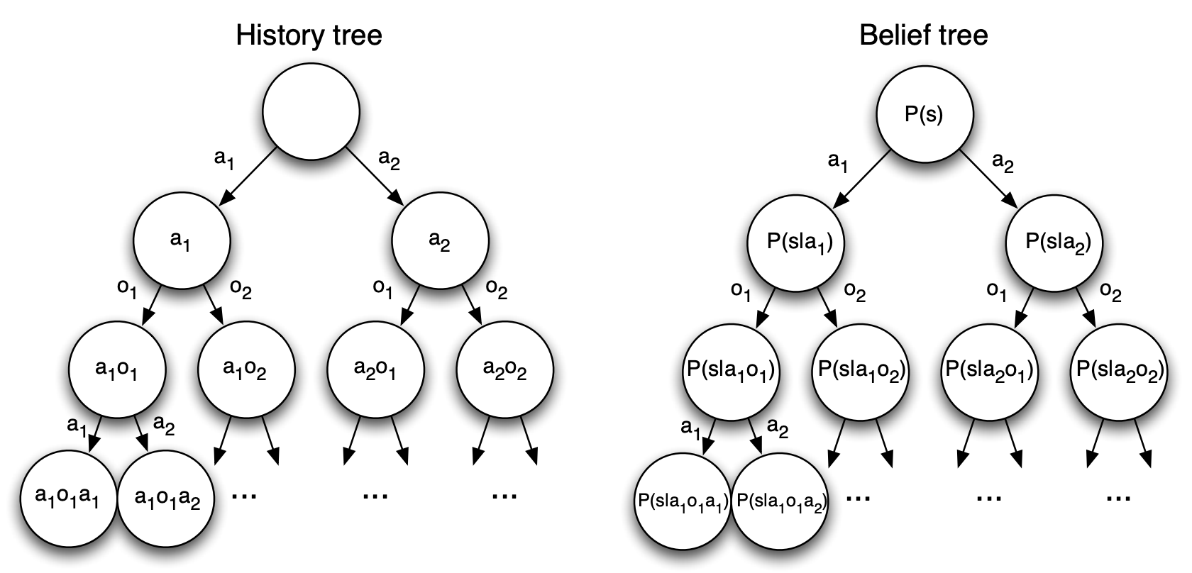
History-based	$H_t = A_0, O_1, R_1, \cdots, O_t, R_t$	Always Markov, but grows unboundedly
Belief-based	$b(h) = [\mathbb{P}(S_t = s^1 \mid H_t), \cdots, \mathbb{P}(S_t = s^n \mid H_t)]$	Compact distribution over states; also Markov

Both history and belief state satisfy the Markov property, so we can treat them as states in a new (larger) MDP:

The catch: this converted MDP has an infinite (or continuous) state space, making it much harder to solve than the original.

Undiscounted, Average Reward MDPs

When Discounting Doesn't Make Sense

For continuing tasks (no terminal state) where we care equally about all time steps, discounting feels arbitrary. Instead, we can optimize the average reward per step.

This requires ergodic MDPs — where every state is visited infinitely often, without periodic patterns. Think of it as: “no matter where you start, you’ll eventually explore everything.”

Definition (Average Reward):

For an ergodic MDP, the average reward $\rho^\pi$ is independent of the starting state:

\[\rho^\pi = \lim_{T \rightarrow \infty} \frac{1}{T} \mathbb{E}\left[\sum_{t=1}^T R_t\right]\]

Average Reward Value Function

Instead of measuring total discounted reward, we measure how much better (or worse) a state is compared to the average:

\[\widetilde{v}_{\pi}(s) = \mathbb{E}_{\pi}\left[\sum_{k=1}^\infty (R_{t+k} - \rho^\pi) \mid S_t = s \right]\]

This leads to an average-reward Bellman equation:

\[\widetilde{v}_{\pi}(s) = \mathbb{E}_{\pi}\left[(R_{t+1} - \rho^\pi) + \widetilde{v}_{\pi}(S_{t+1}) \mid S_t = s \right]\]

Notice the similarity to the standard Bellman equation — we just subtract the baseline $\rho^\pi$ from each reward.

Lecture 3: Planning by Dynamic Programming

Official Lecture Slides

Introduction

What is Dynamic Programming?

• Dynamic refers to the sequential / or temporal component of the problem (changes stepwise).
• Programming refers to optimizing a “program”, i.e. a Policy.

In other words, it’s a method for solving complex problems, by breaking them up into subproblems, solving those and then combining their solutions into the main solution.

Requirements for Dynamic Programming

Dynamic Programming is a very general solution method for problems which have two properties:

• Optimal substructure
  • Principle of optimality applies:

    optimal substructure basically tells you that you can solve some overall Problem by breaking it down into two pieces or more, solving for each of those pieces and that the optimal solution to those pieces tells you how to get the optimal solution to your overall problem.

  • Optimal solution can be decomposed into subproblems
• Overlapping subproblems
  • Subproblems recur many times
  • Solutions can be cached and reused

Markov decision processes satisfy both properties:

• Bellman Equation (expectation & optimality) gives recursive decomposition
• Value function stores and reuses solutions

Planning by Dynamic Programming

Via Dynamic Programming, we aim to solve the planning problem which assumes full knowledge of the MDP:

This does NOT cover the full reinforcement learning problem (where the environment may be initially unknown)

• We are given: state space, action space, transition dynamics, reward function, and discount factor
• Goal: Solve the MDP with perfect knowledge of how the environment works

Two special cases of planning an MDP:

1. Prediction (Policy Evaluation)

   Goal: Evaluate how good a given policy is — determine how much reward we’ll get from any state when following policy $\pi$

   • Input: MDP $\langle \mathcal{S}, \mathcal{A}, \mathcal{P}, \mathcal{R}, \gamma \rangle$ + Policy $\pi$
     • or MRP $\langle \mathcal{S}, \mathcal{P^\pi}, \mathcal{R^\pi}, \gamma \rangle$
   • Output: Value function $v_\pi$

   Example (Atari): Given the game rules and a specific way of playing (policy), calculate expected score from each game state.

2. Control (Optimization)

   Goal: Find the best possible policy, i.e. the mapping from states to actions that achieves maximum long-term reward

   • Input: MDP $\langle \mathcal{S}, \mathcal{A}, \mathcal{P}, \mathcal{R}, \gamma \rangle$
   • Output: Optimal value function \(v_{*}\) (or \(q_{*}\)) + Optimal policy $\pi_*$

   Example (Atari): Given full access to game internals, find the best possible strategy to maximize score.

Approach: We typically solve prediction as a subroutine within control, i.e. via first learning to evaluate policies, then using that to find the optimal one.

Other Applications of Dynamic Programming

Feel free to skim over this subsection / skip it.

Dynamic programming is used to solve many other problems, e.g.

• Scheduling algorithms
• String algorithms (e.g. sequence alignment)
• Graph algorithms (e.g. shortest path algorithms)
• Graphical models (e.g. Viterbi algorithm)
• Bioinformatics (e.g. lattice models)

Policy Evaluation

Definition

• Problem: evaluate a given policy π

• Solution: iterative application of Bellman Expectation Equation:

  \[v_1 \rightarrow v_2 \rightarrow \cdots \rightarrow v_\pi\]
• Using synchronous backups,
  • At each iteration $k + 1$
  • For all states $s \in \mathcal{S}$
  • Update $v_{k+1}(s)$ from $v_{k}(s’)$:
    • where $s’$ is a successor state of $s$.

Asynchronous Backups and Convergence to $v_\pi$ will be discussed later.

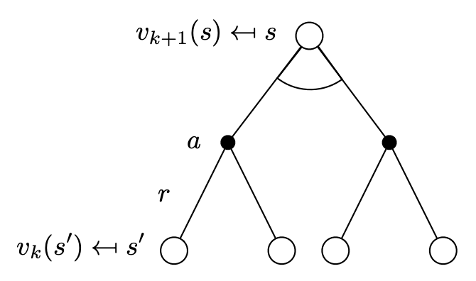
Consider the following backup diagram, which indicates the value function at a given state on iteration step $k+1$, the only difference we see here, compared to the expectation equation diagram is that the value function for next state is taken from the previous iteration step:

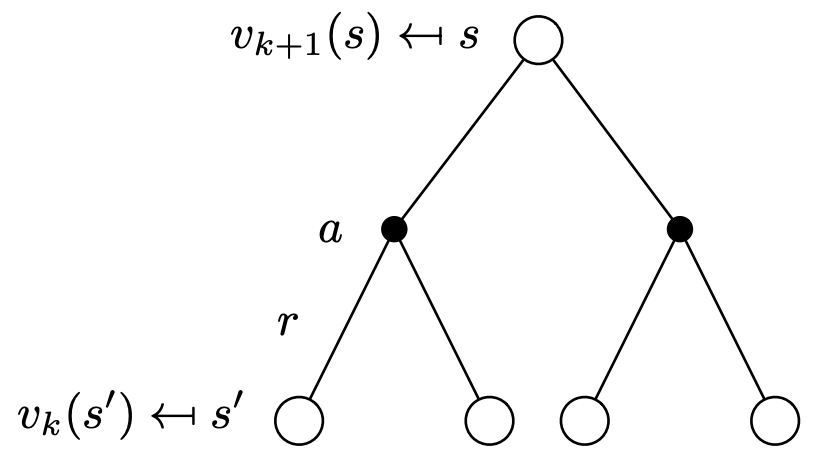
From the above diagram, and previously discussed derivations, we come up with the following recursive equations for:

• MDP (need a referesher?):

  \[v_{k+1}(s) = \sum\limits_{a \in \mathcal{A}}\pi(a\mid S)(R_{s}^a + \gamma \sum\limits_{s' \in \mathcal{S}}\mathcal{P_{ss'}^a} v_{k}(s'))\]

• MRP (need a referesher?):

  \[v_{k+1} = \mathcal{R^\pi} + \gamma\mathcal{P^\pi}\cdot v_{k}\]

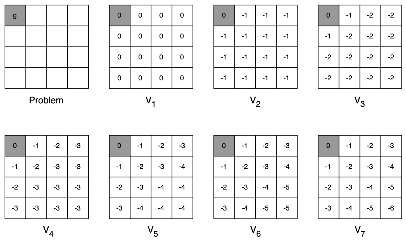
Small Gridworld - Random Policy Example

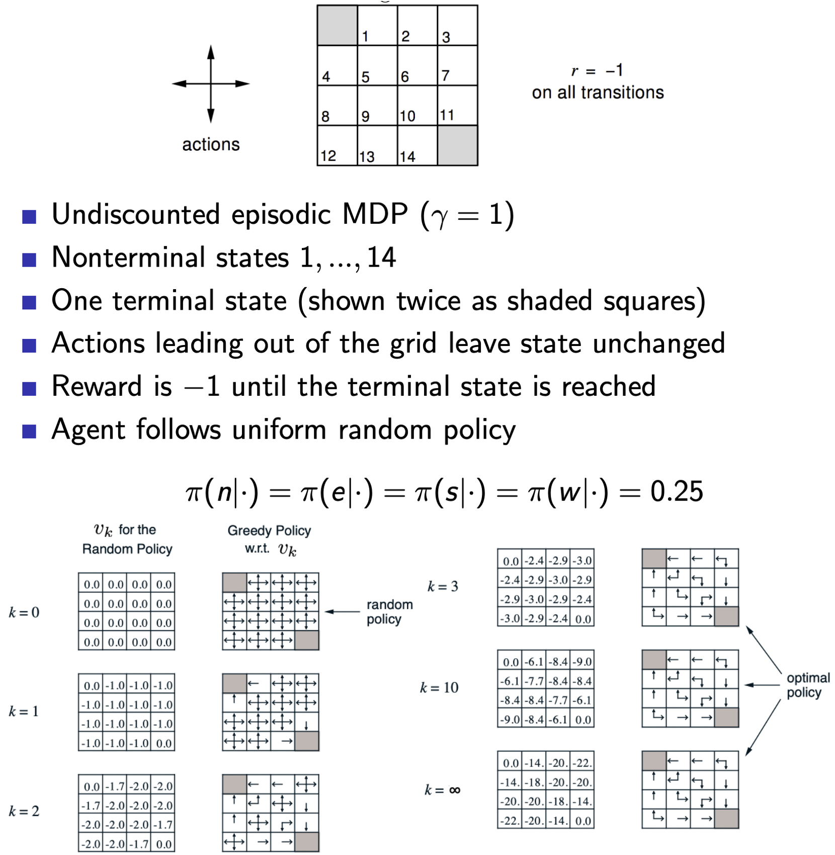Value function helps us figure out better policies. Eventhough we were just evaluating one policy, we can use that to build a new policy by acting greedily!

Policy Iteration

Definition

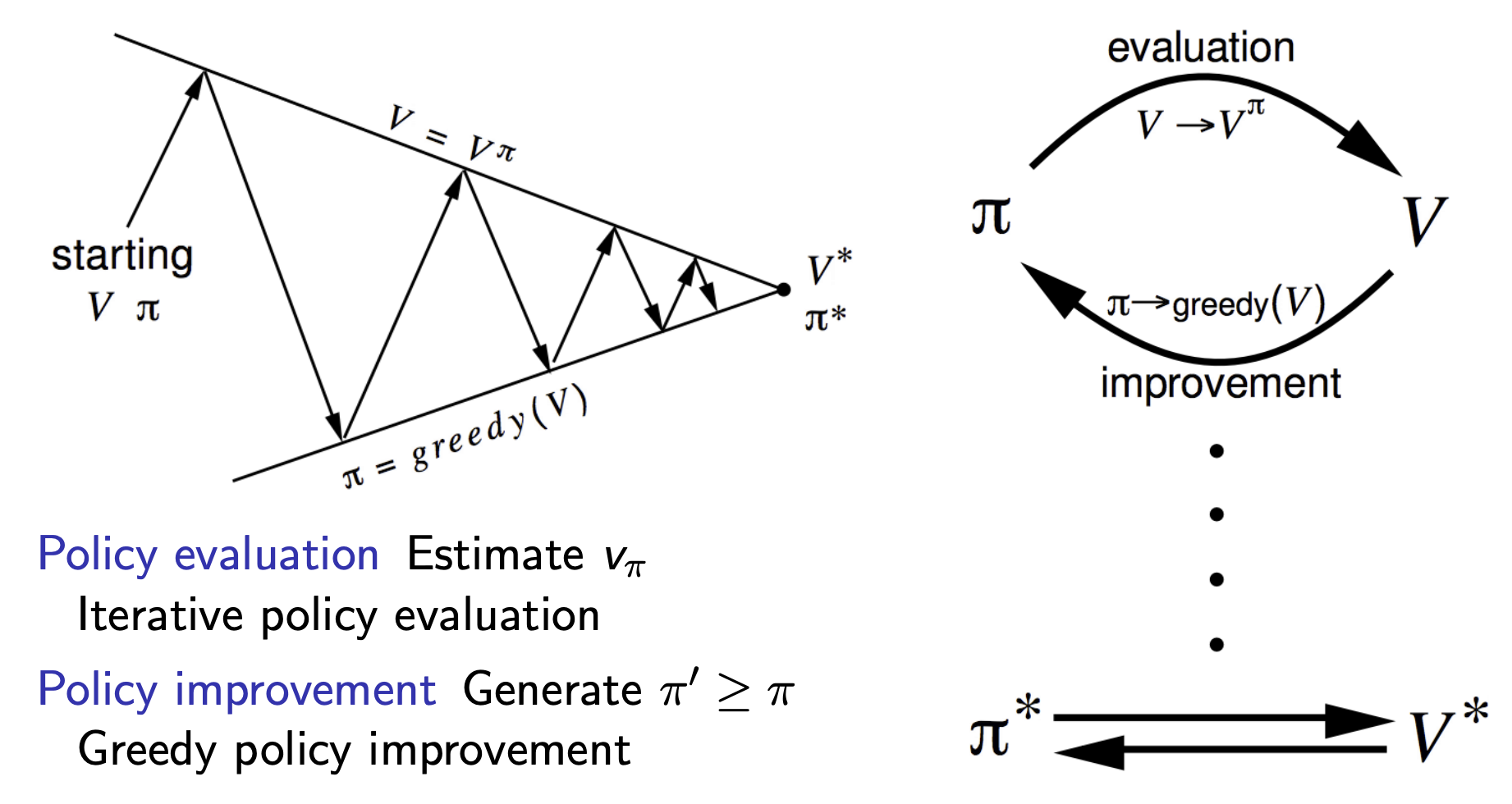
To make a policy better, we’ll first evaluate the policy (as described above), and then improve the policy by acting greedily based on the evaluated value function. We iterate policies using this process recursively.

In other words, given a policy $\pi$

• Evaluate the policy $\pi$:

  \[v_{\pi}(s) = \mathbb{E}[R_{t+1} + \gamma R_{t+2} + \cdots \mid S_t = s]\]

• Improve the policy by acting greedily with respect to $v_\pi$

  \[\pi' = greedy(v_\pi)\]

This process, when run iteratively, always converges to $\pi*$

In our previous example, we just evaluated the policy once and kept iteratively converging on it using the same policy (simultaneously maintaing possible optimial policies on the side which converged to a greedy policy in 3 iterations, much before the value function converged). However, in general cases, we need more iterations of improvement / evaluation.

Example: Jack’s Car Rental

Consider the following scenario:

• States: Two Locations with a capacity of 20 cars each
• Actions: Move upto 5 cars from one location to the other
  • Reward: -2$ for each moved car
• Transitions (Environment Stochasticity): Cars Can be returned and requested randomly

  • Both the request / return for both locations follow the poisson distribution of probability:

    \[\mathbb{P}(n) = \frac{\lambda^n}{n!}e^{-\lambda}\]
    • Location 1: $\text{Return: } \lambda_{ret1} = 3, \text{ Rent: }\lambda_{req1} = 3$
    • Location 2: $\text{Return: } \lambda_{ret2} = 2, \text{ Rent: }\lambda_{req2} = 4$

  • Reward: 10$ for each rented car

For a given policy $\pi(i, j)$, where $i, j \in [0, 20]$ represent car availability in both locations, we can simply define the Bellman Expectation Equation as follows:

\[\begin{aligned} & \text{Let } a = \pi(i, j) \\ & \text{Let } \hat{i} = i - a, \quad \hat{j} = j + a \quad \text{(Inventory after moves)} \\ & \text{Let } r_1 = \min(\hat{i}, \text{req}_1), \quad r_2 = \min(\hat{j}, \text{req}_2) \quad \text{(Actual rentals)} \\ \\ V_\pi(i, j) &= \underbrace{-2|a|}_{\text{Deterministic Cost}} \\ & \quad + \sum_{\text{req}, \text{ret}} P(\text{req}, \text{ret}) \Bigg[ \underbrace{10(r_1 + r_2)}_{\text{Rental Reward}} + \gamma V\Big( \text{clamp}(\hat{i} - r_1 + \text{ret}_1), \text{clamp}(\hat{j} - r_2 + \text{ret}_2) \Big) \Bigg] \\ & \text{Where } P(\text{req}, \text{ret}) = \underbrace{\frac{\lambda_{req1}^{k_1}}{k_1!}e^{-\lambda_{req1}}}_{P(req_1=k_1)} \times \underbrace{\frac{\lambda_{req2}^{k_2}}{k_2!}e^{-\lambda_{req2}}}_{P(req_2=k_2)} \times \underbrace{\frac{\lambda_{ret1}^{m_1}}{m_1!}e^{-\lambda_{ret1}}}_{P(ret_1=m_1)} \times \underbrace{\frac{\lambda_{ret2}^{m_2}}{m_2!}e^{-\lambda_{ret2}}}_{P(ret_2=m_2)} \end{aligned}\]

The above can then be used to iteratively update the value function, which can then be used to build a greedy policy and so on and so forth! The below illustration depicts convergance of the policy as we follow this process: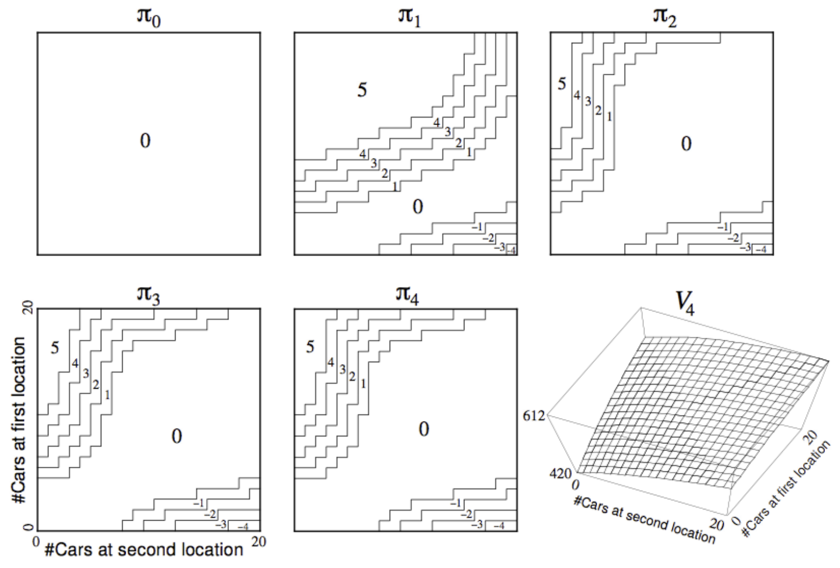

Proof: The Policy Improves!

As after a step of acting greedily, we are stuck with a deterministic policy (it might be stochastic if we choose to keep multiple possible actions with maximal actions-values, but for this case let’s consider we only keep 1), thus we may as well just start with a random deterministic policy: $a = \pi(s)$

• Now, from our definition we can improve this policy by acting greedily wrt to its value function

  \[\pi'(s) = \underset{a \in \mathcal{A}}{\text{argmax}}\ q_\pi(s, a)\]

• At the very least we can say that as this chooses the action resulting in the maximum action-value, it improves our policy for one step. So say from each state, the next step we take is based on this updated policy $\pi’$, and there on we continue following our original policy $\pi$, we get:

  \[q_\pi(s, \pi'(s)) = \underset{a \in \mathcal{A}}{\text{argmax}}\ q_\pi(s, a) \geq q_\pi(s, \pi(s)) = v_\pi(s)\]

• Recursively applying this understanding, we eventually get: \(\begin{aligned} v_\pi(s) &\leq q_\pi(s, \pi'(s)) = \mathbb{E_{\pi'}}\left[R_{t+1} + \gamma v_\pi(S_{t+1}) \mid S_t = s\right] \\ &\leq \mathbb{E_{\pi'}}\left[R_{t+1} + \gamma q_\pi(S_{t+1}, \pi'(S_{t+1})) \mid S_t = s\right]\\ &\leq \mathbb{E_{\pi'}}\left[R_{t+1} + \gamma R_{t+2} \gamma^2 q_\pi(S_{t+2}, \pi'(S_{t+2})) \mid S_t = s\right] \\ &\leq \mathbb{E_{\pi'}}\left[R_{t+1} + \gamma R_{t+2} \gamma^2 q_\pi(S_{t+2}, \pi'(S_{t+2})) \cdots \mid S_t = s\right] = v_{\pi_*}(s) \end{aligned}\)

  or to put simply, \(v_\pi(s) \leq v_{\pi_*}(s)\), the policy improves!

• This improvement can be done iteratively, and stops when:

  \[q_\pi(s, \pi'(s)) = \underset{a \in \mathcal{A}}{\text{argmax}}\ q_\pi(s, a) \textcolor{pink}{\textbf{=}} q_\pi(s, \pi(s)) = v_\pi(s)\]

• or, simply:

  \[\underset{a \in \mathcal{A}}{\text{argmax}}\ q_\pi(s, a) = v_\pi(s)\]

  Look familiar? That’s the Bellman Optimality Equation for MDPs, and as it’s been satisified! we can safely say that:

  \[v_\pi(s) = v_{*}(s) \ \forall \ s\]

• Policy $\pi$ is optimal.

Does Policy Evaluation Need to Converge?

Revisiting our grid world example again, we notice that to reach the final greedy policy our value function really didn’t have to converge, we got the policy right at $k=3$. So now the question is, Does policy evaluation really need to converge to $v_\pi$? It turns out not, we can go with the following Modified Policy Iteration Methods:

• Should we introduce a stopping condition (e.g. $\epsilon$ convergence of value function)
• Simply stop after $k$ iterations of the iterative policy evaluation step ?
  • What if we update policy every iteration? i.e. $k=1$?
    • This is equivalent to Value Iteration (coming up next!)

Value Iteration

Principle of Optimality

As we already know, any optimal policy can be subdivided into:

• An optimal first action $A_*$
• Followed by an optimal policy from successor state $S’$

Theorem (Principle of Optimality)

A policy $\pi(a \mid s)$ achieves the optimal value from state $s$, \(v_\pi(s) = v_{*}(s)\), if and only if

• For any state $s’$ reachable from $s$
• $\pi$ achieves the optimal value from state $s’$, \(v_\pi(s') = v_{*}(s')\)

Deterministic Value Iteration

• If we know the solution to subproblems $v_{*}(s’)$

• Then solution $v_{*}(s)$ can be found by one-step lookahead

  \[v_{*}(s) \leftarrow \underset{a \in \mathcal{A}}{\text{max}} \ \mathcal{R_s^a} + \gamma \sum_{s' \in \mathcal{S}}\mathcal{P_{ss'}^a}v_{*}(s')\]
• Or in other words we can apply the bellman optimality equation iteratively to update the value function making it reach its optimal value:
  • We start with a randomly initialized value function $v_1$

  • We iteratively apply Bellman Optimality Backup to improve the value function:

    \[v_1 \rightarrow v_2 \rightarrow \cdots \rightarrow v_{*}\]

    using synchronus backups, i.e. at each iteration $k$:

    we update $v_k(s) \ \text{from} \ v_{k-1}(s’)$ $\forall s \in \mathcal{S}$

  • An important thing to note here is that unlike Policy Iteration, we don’t have any explicit policy here, in fact intermediate value functions may not even correspond to any policy!
  • Also note from previous section, that this is techinically equivalent to modified policy iteration with $k=1$.

  • The following backup diagram illustrates the above mentioned process

    

    Mathematically, the above is equivalent to:

    \[\begin{aligned} & v_{k+1}(s) \leftarrow \underset{a \in \mathcal{A}}{\text{max}} \ \mathcal{R_s^a} + \gamma \sum_{s' \in \mathcal{S}}\mathcal{P_{ss'}^a}v_{k}(s') \\ & \mathbf{v}_{k+1} \leftarrow \underset{a \in \mathcal{A}}{\text{max}} \ \left(\mathcal{R^a} + \gamma \mathbf{\mathcal{P^a}v_{k}}\right) \end{aligned}\]

• A simple intuition for this is imagining the process as starting with final rewards (say there’s an end / goal state) and working backwards. Here’s an illustrated example for a problem where we are trying to find the shortest path of all cells from the top-left corner (goal state).

  

  Q. In the shortest path example, the value function values keep getting more negative (smaller). But didn’t we prove that values improve during policy iteration?

  Ans. This question highlights a key difference between policy iteration and value iteration:

  • The theorem showing values getting “better” was for policy iteration, not value iteration.
  • In value iteration, the intermediate values $v_k$ may not correspond to any actual policy; they’re just stepping stones toward $v_{*}$.
  • If you were to fully evaluate a policy at each step of policy iteration and then compare it to the greedy-improved policy, yes, the value function would strictly improve.
  • But in value iteration, we never claimed the intermediate values are monotonically increasing; only that they converge to the optimal value function.

  The confusion arises because:

  • Policy iteration: We evaluate real policies $\rightarrow$ values of successive policies improve
  • Value iteration: We’re not evaluating real policies $\rightarrow$ intermediate values just converge to $v_{*}$

It’s important to note that in practice the algorithm doesn’t even know that a final State exists, even if there is no final State the algorithm will still work. Even if the mdp is ergodic and just goes on forever continuing, or an mdp that has some discount factor and just goes on forever: Dynamic Programming still works. It will still find the optimal solution. There could in fact be one, many or no goal state at all.

A great example of value iteration in practice

This link is different than the one given by David in the lecture as that no longer works in most modern browsers, but you don’t have to worry about it, this one’s made by Andrej Karpathy

Summary of DP Algorithms

Synchronous Dynamic Programming Algorithms

Problem	Bellman Equation	Algorithm
Prediction	Bellman Expectation Equation	Iterative Policy Evaluation
Control	Bellman Expectation Equation + Greedy Policy Improvement	Policy Iteration
Control	Bellman Optimality Equation	Value Iteration

• Algorithms are based on state-value function $v_\pi(s)$ or $v_{*}(s)$
  • Complexity $O(mn^2)$ per iteration, for $m$ actions and $n$ states
• Could also apply to action-value function $q_\pi(s, a)$ or $q_*(s, a)$
  • Complexity $O(m^2n^2)$ per iteration

Extensions to Dynamic Programming

Asynchronous Dynamic Programming

DP methods described so far used synchronous backups, i.e. all states are backed up in parallel. Asynchronous DP on the other hand, backs up states individually, in any order:

• For each selected state, apply the appropriate backup.
• This can significantly reduce computation and is Guaranteed to converge if all states continue to be selected.

Three Simple Ideas for Asynchronous DP

1. In-Place Dynamic Programming

• Synchronous DP stores 2 versions of the value function:

  $\forall s \in S$

  \[\textcolor{pink}{v_{new}(s)} \leftarrow \underset{a \in \mathcal{A}}{\text{max}} \ \mathcal{R_s^a} + \gamma \sum_{s' \in \mathcal{S}}\textcolor{pink}{\mathcal{P_{ss'}^a}v_{old}(s')}\]

• Asynchronous DP stores just 1 version:

  $\forall s \in S$

  \[\textcolor{pink}{v(s)} \leftarrow \underset{a \in \mathcal{A}}{\text{max}} \ \mathcal{R_s^a} + \gamma \sum_{s' \in \mathcal{S}}\textcolor{pink}{\mathcal{P_{ss'}^a}v(s')}\]

  Note that here, the ordering in which these states are updated, really matters, consider a specific scenario where we are given a goal state and we iterate backwards to the states branching out of it, the updates would be much more efficient as compared to iterating from leaf states back to the goal state. This ordering optimality motivates the next approach:

2. Prioritised Sweeping

• Use magnitude of Bellman error to guide state selection, e.g

  \[\left|\underset{a \in \mathcal{A}}{\text{max}} \left(\mathcal{R_s^a} + \gamma \sum_{s' \in \mathcal{S}}\mathcal{P_{ss'}^a}v(s')\right) - v(s)\right|\]
• Backup the state in decreasing order of Bellman error (implemented efficiently via priority queue), this error of affected states is updated after each backup.
• Requires knowledge of reverse dynamics (predecessor states)

3. Real-Time Dynamic Programming

The idea of real-time dynamic programming is to select the states that the agent actually visit. Instead of just sweep over everything naively, we actually run an agent in the real world, collect real samples / random samples from some real trajectory and update around those real samples. So say if an agent is wandering around a specific section of a grid, we care much more about those specific states than what’s going on in the far corner of the grid, because that’s what the agent is actually encountering under its current policy. Simply put, the idea is to:

• Use agent’s experience to guide the selection of states
• After each time-step \(S_t, A_t, R_{t+1}\)

• Backup the state $S_t$

  \[\textcolor{pink}{v(S_t)} \leftarrow \underset{a \in \mathcal{A}}{\text{max}} \ \mathcal{R_{\textcolor{pink}{S_t}}^a} + \gamma \sum_{s' \in \mathcal{S}}\textcolor{pink}{\mathcal{P_{S_t s'}^a}v(s')}\]

Full-Width vs Sample Backups

Full-Width Backups (DP)

Dynamic programming uses full-width backups: for each state update, we consider:

• All actions (max over the entire action space)
• All successor states (weighted by transition probabilities)

This has two major drawbacks:

1. Expensive: We enumerate the full branching factor at every step
2. Requires a model: We need to know the transition dynamics $\mathcal{P}_{ss’}^a$

Sample Backups (Preview of Model-Free RL)

Instead of exhaustive enumeration, we can sample trajectories $\langle S, A, R, S’ \rangle$ and estimate expectations from these samples.

Aspect	Full-Width Backup	Sample Backup
Computation	$O(|A| \cdot |S|)$ per state	$O(1)$ per sample
Model required?	Yes	No
Scalability	Fails for large MDPs	Works well for large MDPs

Key insight: By sampling transitions from the environment (rather than computing over all possibilities), we:

• Break the curse of dimensionality
• Eliminate the need to know the model

This is the bridge from dynamic programming (model-based planning) to model-free reinforcement learning (covered in upcoming lectures).

Approximate Dynamic Programming

Even with sample backups, we still need to store a value for every state. For truly massive state spaces (continuous states, high-dimensional observations), this becomes infeasible. The solution: approximate the value function using a parameterized function.

Function Approximation

Instead of storing $v(s)$ for each state, we use a function approximator:

\[\hat{v}(s, \mathbf{w}) \approx v(s)\]

where $\mathbf{w}$ is a parameter vector (e.g., weights of a neural network). We then apply dynamic programming to this approximate value function.

Fitted Value Iteration

A concrete example of approximate DP. At each iteration $k$:

1. Sample states: Select a subset $\tilde{\mathcal{S}} \subseteq \mathcal{S}$

2. Compute targets: For each sampled state $s \in \tilde{\mathcal{S}}$, estimate the target value using the Bellman optimality equation:

   \[\tilde{v}_k(s) = \underset{a \in \mathcal{A}}{\text{max}} \left( \mathcal{R}_s^a + \gamma \sum_{s' \in \mathcal{S}} \mathcal{P}_{ss'}^a \hat{v}(s', \mathbf{w}_k) \right)\]

3. Train the approximator: Fit the next value function $\hat{v}(\cdot, \mathbf{w}_{k+1})$ using the collected targets ${(s, \tilde{v}_k(s))}$ as a supervised learning problem.

This combines the ideas of sampling (don’t enumerate all states) and function approximation (don’t store values for all states) — essential ingredients for scaling RL to real-world problems.

Contraction Mapping

This section provides the theoretical foundation for why DP algorithms converge. The key questions we answer:

• How do we know value iteration converges to $v_*$?
• How do we know iterative policy evaluation converges to $v_\pi$?
• Is the solution unique?
• How fast do these algorithms converge?

Value Function Space

Consider the vector space $\mathcal{V}$ over value functions:

• There are \(\| \mathcal{S} \|\) dimensions (one per state)
• Each point in this space fully specifies a value function $v(s)$

Key question: What does a Bellman backup do to points in this space?

We will show that it brings value functions closer together, and therefore the backups must converge to a unique solution.

Value Function $\infty$-Norm

We measure distance between state-value functions $u$ and $v$ using the $\infty$-norm (max norm):

\[\|u - v\|_\infty = \underset{s \in \mathcal{S}}{\text{max}} \ |u(s) - v(s)|\]

This captures the largest difference between any two state values.

Bellman Expectation Backup is a Contraction

What is the Bellman Backup Operator?

Recall that in iterative policy evaluation, we repeatedly apply the Bellman expectation equation to update our value function. We can think of this update as an operator: a function that takes one value function and produces another.

Define the Bellman expectation backup operator $T^\pi$:

\[T^\pi(v) = \mathcal{R}^\pi + \gamma \mathcal{P}^\pi v\]

What does this mean? Given any value function $v$, applying $T^\pi$ produces a new value function by:

1. Taking the expected immediate reward $\mathcal{R}^\pi$ under policy $\pi$
2. Adding the discounted ($\gamma$) expected value of successor states ($\mathcal{P}^\pi v$)

This is exactly what we do in each iteration of policy evaluation, we’re just writing it compactly as an operator.

What is a Contraction?

Intuitively, a contraction is an operator that brings things closer together. Imagine two different value function estimates $u$ and $v$ as two points in space. If we apply a contraction operator to both, the resulting points $T(u)$ and $T(v)$ will be closer to each other than $u$ and $v$ were originally.

More precisely, a $\gamma$-contraction satisfies:

\[\|T(u) - T(v)\| \leq \gamma \|u - v\| \quad \text{where } \gamma < 1\]

The distance after applying $T$ is at most $\gamma$ times the original distance. Since $\gamma < 1$, the distance shrinks with each application.

Proving $T^\pi$ is a $\gamma$-Contraction

Let’s show that no matter which two value functions $u$ and $v$ we start with, applying $T^\pi$ to both brings them closer:

\[\begin{aligned} \|T^\pi(u) - T^\pi(v)\|_\infty &= \|(\mathcal{R}^\pi + \gamma \mathcal{P}^\pi u) - (\mathcal{R}^\pi + \gamma \mathcal{P}^\pi v)\|_\infty \\ &= \|\gamma \mathcal{P}^\pi (u - v)\|_\infty && \text{(rewards cancel out)} \\ &\leq \|\gamma \mathcal{P}^\pi\| \|u - v\|_\infty && \text{(norm property)} \\ &\leq \gamma \|u - v\|_\infty && \text{(since } \|\mathcal{P}^\pi\| \leq 1 \text{)} \end{aligned}\]

Why is $|\mathcal{P}^\pi| \leq 1$? Because $\mathcal{P}^\pi$ is a stochastic matrix (rows sum to 1). Multiplying by it computes a weighted average, which can never increase the maximum value, ergo it can only shrink or preserve it.

The key insight: The discount factor $\gamma < 1$ is doing the heavy lifting here. Every time we apply $T^\pi$, we multiply the “difference” between value functions by $\gamma$, guaranteeing it shrinks.

Contraction Mapping Theorem

Now we can state the powerful theorem that guarantees convergence:

Theorem (Contraction Mapping Theorem):

For any metric space $\mathcal{V}$ that is complete (i.e., closed) under an operator $T(v)$, where $T$ is a $\gamma$-contraction:

• $T$ converges to a unique fixed point
• At a linear convergence rate of $\gamma$

Why does this guarantee convergence? Think about it this way:

• Start with any initial guess $v_0$
• Apply $T$ repeatedly: $v_1 = T(v_0)$, $v_2 = T(v_1)$, …
• Each application shrinks the distance to the true solution by factor $\gamma$
• After $k$ iterations, the error is at most $\gamma^k$ times the initial error
• Since $\gamma < 1$, this goes to zero as $k \to \infty$

Why is the fixed point unique?

If there were two fixed points \(v^{*}\) and \(u^{*}\), then:

• \(T(v^{*}) = v^{*}\) and \(T(u^{*}) = u^{*}\). But the contraction property says \(\|T(v^{*}) - T(u^{*})\| \leq \gamma \|v^{*} - u^{*}\|\), which means:
• \(\|v^{*} - u^{*}\| \leq \gamma \|v^{*} - u^{*}\|\).

Since \(\gamma < 1\), this is only possible if \(\|v^{*} - u^{*}\| = 0\), i.e., they’re the same point.

Convergence of Policy Evaluation & Policy Iteration

Applying the contraction mapping theorem to the Bellman expectation operator:

• The Bellman expectation operator $T^\pi$ has a unique fixed point
• $v_\pi$ is a fixed point of $T^\pi$ (by Bellman expectation equation)
• By the contraction mapping theorem:
  • Iterative policy evaluation converges to $v_\pi$
  • Policy iteration converges to $v_*$

Bellman Optimality Backup is a Contraction

Define the Bellman optimality backup operator $T^*$:

\[T^*(v) = \underset{a \in \mathcal{A}}{\text{max}} \ \mathcal{R}^a + \gamma \mathcal{P}^a v\]

This operator is also a $\gamma$-contraction (proof similar to above):

\[\|T^*(u) - T^*(v)\|_\infty \leq \gamma \|u - v\|_\infty\]

Convergence of Value Iteration

Applying the contraction mapping theorem to the Bellman optimality operator:

• The Bellman optimality operator $T^*$ has a unique fixed point
• \(v_*\) is a fixed point of \(T^*\) (by Bellman optimality equation)
• By the contraction mapping theorem:
  • Value iteration converges to $v_*$

Lecture 4: Model-Free Prediction

Official Lecture Slides

Introduction

• In the previous lecture we discussed Dynamic Programming methods to solve a known MDP (i.e. dynamics of the agent’s environment were known).
• In this lecture we discuss Model-Free Prediction, which applies to cases where we try to evaluate a given policy by estimating its value function in an unknown MDP, i.e., when the dynamics of the environment are unknown.
• In the next lecture, we build on this by talking about Model-Free Control, which helps us find the optimal value function and hence the optimal policy without knowing the environment model.

Monte-Carlo Learning

MC (Monte-Carlo) RL methods apply only to episodic MDPs (i.e. all episodes must terminate, ex: A Game) and learn directly from complete episodes (no bootstrapping) of experience. They work on the basic principle of averaging returns observed over episodes for the value of each visited state.

Policy Evaluation

So, the agent’s goal is to learn $v_\pi$ from episodes of experience observed, when it follows a given policy $\pi$. As we’re already familiar with, An episode generated by following policy $\pi$ looks like:

\[S_1, A_1, R_2, S_2, A_2, R_3, \cdots, S_T\]

or simply: \((S_1, A_1, R_2, S_2, A_2, R_3, \cdots, S_T) \sim \pi\)

Also, recall that:

• For a timestep $t$ in this episode, we’d then define the return as:

  \[G_t = R_{t+1} + \gamma R_{t+2} + \cdots + \gamma^{T-t-1}R_{T}\]

  where, $T$ denotes the last timestep of the episode. (this is a forward looking calculation, i.e. the expected return is calculated for each visited state once the episode ends)

• And then over all observed episodes, for each visited state $s$, we might define the value function (expected return) as:

  \[v_{\pi}(s) = \mathbb{E}_{\pi}[G_t | S_t = s]\]

  Monte-Carlo methods estimate this by computing the empirical mean of observed returns from visits to state s.

First-Visit Monte-Carlo Policy Evaluation

• In each episode, the first time-step $t$ that a state $s$ is visited, we:
  • Increment the counter $N(s) \leftarrow N(s) + 1$
  • Increment total return $S(s) \leftarrow S(s) + G_t$

  (Note that these counters accumulate across episodes.)

• The Value is then estimated by the mean return $V(s) = \frac{S(s)}{N(s)}$
• And, as applied by the law of large numbers, $V(s) \rightarrow v_{\pi}(s)$ as $N(s) \rightarrow \infty$

Every-Visit Monte-Carlo Policy Evaluation

• In each episode, for every time-step $t$ that a state $s$ is visited, we:
  • Increment the counter $N(s) \leftarrow N(s) + 1$
  • Increment total return $S(s) \leftarrow S(s) + G_t$

  (As an example, imagine an episode, where we loop back to a state $s_i$ multiple times, then for each visit we increment the counter and the total return is updated with the return calculated from each visit onwards to the episode’s end)

• The Value is then estimated by the mean return $V(s) = \frac{S(s)}{N(s)}$
• Again, $V(s) \rightarrow v_{\pi}(s)$ as $N(s) \rightarrow \infty$

Blackjack Example

Here’s a brief explanation of how Blackjack works if it helps to understand this example.

$\mathcal{S}$ States (200):

• Current Sum (12 - 21): (States below 12 are ignored, as we automatically select the twist action if sum of cards $<12$.)
• Dealer’s Showing Card (ace-10)
• Usable Ace (yes-no)

$\mathcal{A}$ Actions:

• Stick: Stop receiving cards (and terminate)
• Twist: Take another card (no replacement)

$\mathcal{R}$ Rewards:

• For Stick Action:
  • $+1$ if sum of cards > sum of dealer cards
  • $0$ if sum of cards = sum of dealer cards
  • $-1$ if sum of cards < sum of dealer cards
• For Twist Action:
  • $-1$ if sum of cards $> 21$ (and terminate)
  • $0$ otherwise

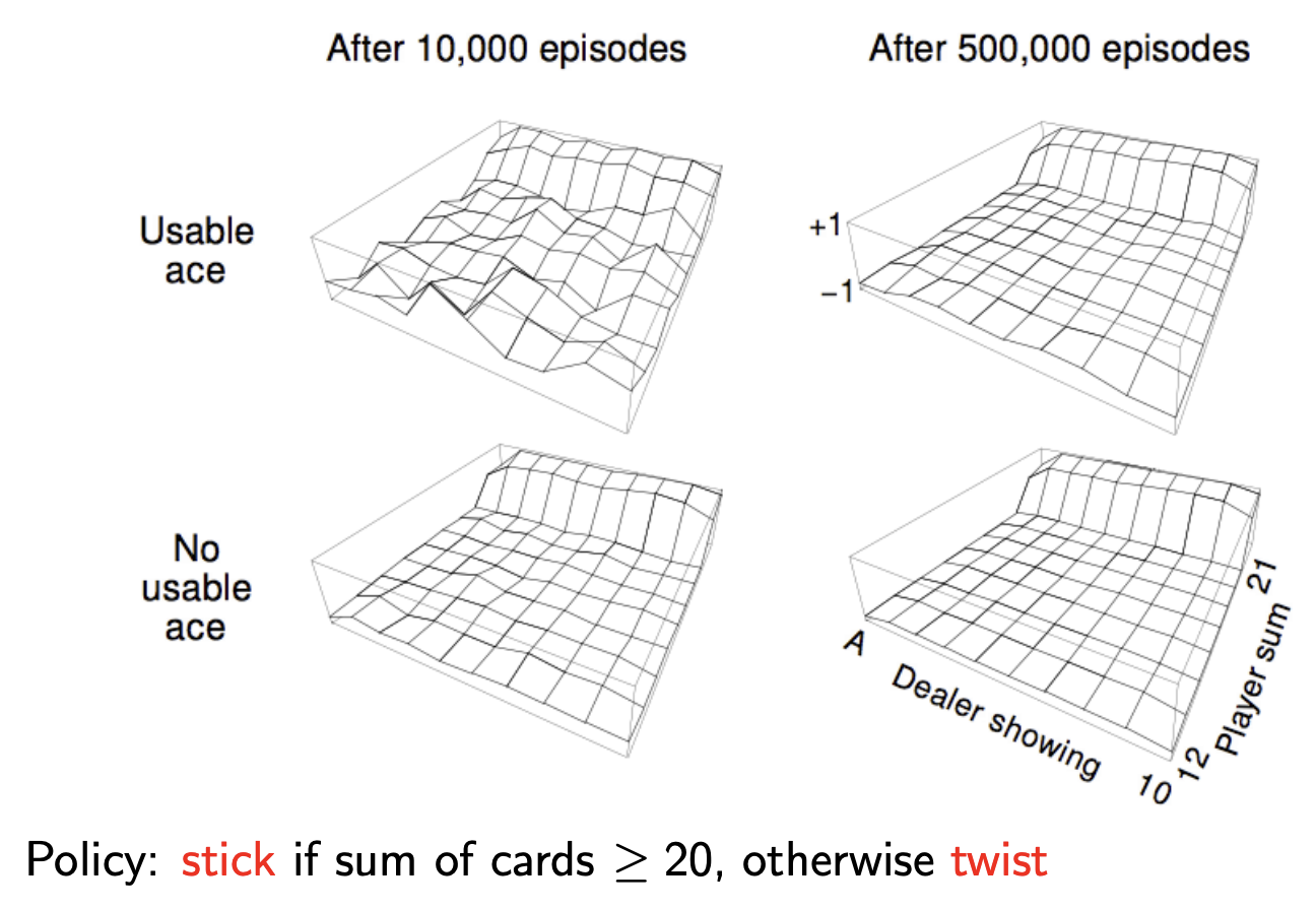
Monte Carlo Policy Evaluation - Blackjack Example: Above, we evaluate a naive policy (stick if sum ≥ 20, otherwise twist) using every-visit MC learning. Post 10K episodes, value function estimates converge for common states, but states with usable aces remain noisy due to rarity. After 500,000 episodes, the true value function emerges, revealing that the naive policy performs poorly except when holding 20 or 21. A key insight from this example is that, while the value function is affected by countless factors—dealer strategy, deck composition, card probabilities, game dynamics; Yet we don’t need explicit knowledge of any of these factors. Through pure trial-and-error sampling of returns, Monte Carlo learning discovers the correct value function directly from experience, demonstrating the power of model-free reinforcement learning!

Incremental Monte-Carlo

Incremental Mean

Till now we’ve been calculating the mean explicitly, i.e. we effectively calculate it post gathering returns and count for all tracked visits for each state. However, this can be done on the fly too, we can keep an online track of the metric as and when we gather values. The incremental calculation can be done as shown below:

\[\begin{aligned} \mu_k &= \frac{1}{k}\sum_{j=1}^k x_j \\ &= \frac{1}{k}\left(x_k + \sum_{j=1}^{k-1}x_j\right) \\ &= \frac{1}{k}\left(x_k + (k-1)\mu_{k-1}\right) \\ &= \mu_{k-1} + \frac{1}{k}\left(x_k -\mu_{k-1}\right) \end{aligned}\]

Incremental Monte-Carlo Updates

• Instead of tracking incremental return & counter and then calculating the mean once all episodes are covered, we can now instead update the value function incrementally:

  • For each state $S_t$ with return $G_t$:

    \[\begin{aligned} N(S_t) \leftarrow N(S_t) + 1 \\ V(S_t) \leftarrow V(S_t) + \frac{1}{N(S_t)}\left(G_t - V(S_t)\right) \end{aligned}\]

    Another perspective of looking at the above result is that we are updating the mean estimate (or $V(S_t)$) a small amount ($\frac{1}{k} * \text{difference}$) towards the observed value of return from that particular time step for the given state

• In non-stationary problems (where weighing much older estimates equally to the current ones slows down the convergence, acting as an unnecessary baggage: a good example would be an environment which gradually changes its dynamics), it can be useful to track a running mean, i.e. forget old episodes.

  \[V(S_t) \leftarrow V(S_t) + \alpha\left(G_t - V(S_t)\right)\]

  Here, instead of keeping a track of number of steps for each state, we have a constant step size ($\alpha$) which gives us an exponential forgetting rate when we’re computing our mean, or in other words the exponential moving average of all of the returns we’ve seen for the state so far.

Temporal-Difference Learning

Similar to MC Learning, Temporal-Difference (TD for short) methods learn directly from episodes of experience (non-episodic experiences as well) and are model-free. Unlike MC methods, TD methods do not require complete episodes. Instead, they update value estimates by bootstrapping, i.e., by using current estimates of successor states.

$\text{TD}(0)$

• Goal: learn $v_\pi$ online from experience under a policy $\pi$

• The simplest temporal-difference learning algorithm $\text{TD}(0)$, works by updating the value of a state using the immediate reward and the estimated value (discounted) of the next state:

  \[V(S_t) \leftarrow V(S_t) + \alpha\left(\textcolor{pink}{R_{t+1} + \gamma V(S_{t+1})} - V(S_t)\right)\]

  Here,

  • \(R_{t+1} + \gamma V(S_{t+1})\), is referred to as TD Target
  • and, \(R_{t+1} + \gamma V(S_{t+1}) - V(S_t)\), is referred to as the TD Error

• Why TD? An example:

  Consider the following scenario: You’re driving and you see suddenly a car that comes hurtling towards you. You think you’re going to crash, but then you don’t actually crash, at the last second the car swerves out of the way:

  • In Monte Carlo you wouldn’t get this negative reward, i.e. you wouldn’t have a crash, ergo you wouldn’t be able to update your value to say that you almost died. But in:
  • TD learning you’re in this situation where you think everything’s fine and then on the next timestep you’re now in a situation where you think you’re going to die (i.e. a car crash is going to happen). And so you can immediately update the value we had before to say oh that was actually worse than I thought maybe I should have slowed down the car and anticipated this potential near-death experience (which can be done immediately in TD, as we don’t need to wait until the crash happens / you die to update our value function).

Driving Home Example

State	Elapsed Time (minutes)	Predicted Time to Go	Total Time
leaving office	0	30	30
reach car, raining	5	35	40
exit highway	20	15	35
behind truck	30	10	40
home street	40	3	43
arrive home	43	0	43

Consider the above story, where at each step we have:

• “Predicted time to go”: how long before the subject reaches home
• Elapsed Time (minutes): How long has it been since we left office?
• Total time: how much total time we do estimate we’ll take to reach home based on the states seen up till now (or current state thinking of this as an MDP).

As can be seen the estimates fluctuate as the subject encounters unexpected events (which may not be regular occurences) such as rain or getting stuck behind the truck / traversing the highway faster than expected.

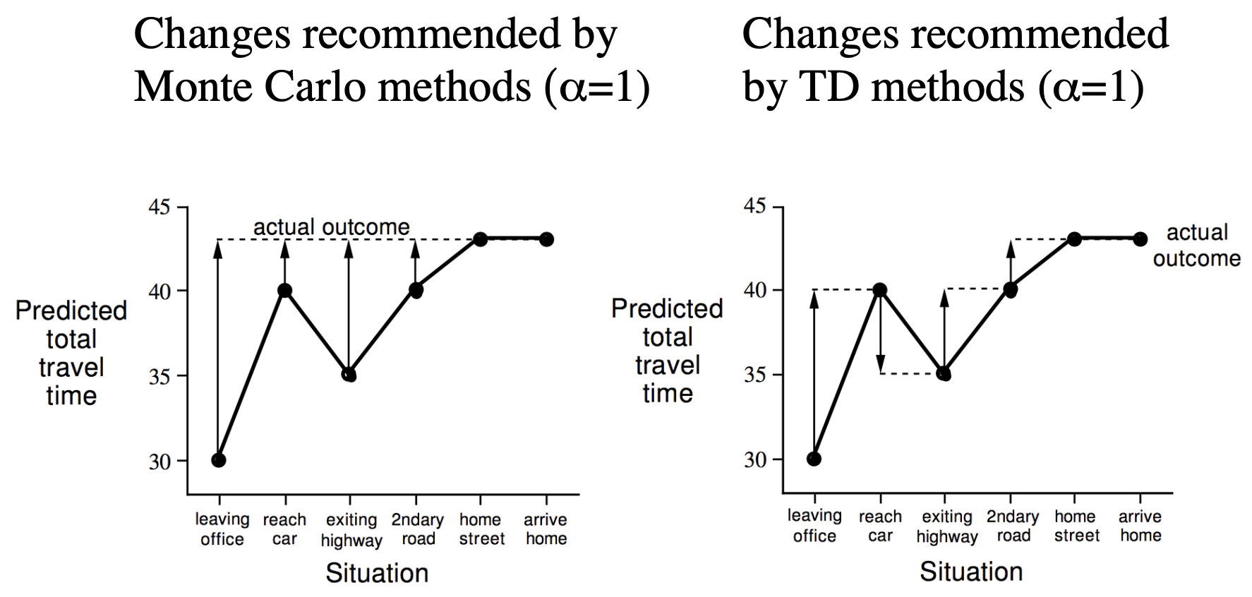
When we apply MC / TD learning to the above estimates of Total Time (as can be seen in the above figure), notice that for:

• Monte-Carlo (MC): All estimates get pushed towards the final true reward (in this case time it took to actually reach home) 43 minutes, which pulls estimates for all states upwards. Indirectly, it increased expected value for “reach car” state due to the later traffic jam (failing to integrate the fact that the immediate reward: drive on the highway was actually faster!).
• Temporal-Difference (TD(0) in this case): As each state’s estimate depends on the immediate reward and expected value of next state (note that because we’re tracking total traversed time, we’ll also add already traversed time to this value to get “Total Time” = Expected “total time” value of next State), notice that the expected value from “reach car” state actually went down acknowledging the fact that the drive on the highway was infact faster!

MC vs TD

Advantages & Disadvantages (1)

• TD can learn before knowing the final outcome:
  • TD can learn online after every step
  • MC must wait untill the end of the episode before the total return is known (which is needed to update each step: learning).
• TD can learn without the final outcome
  • TD can learn from incomplete sequences
  • MC can only learn from complete sequences
  • TD works in continuing (non-terminating) environments
  • MC only works for episodic (terminating) environments

    We can choose to go for some arbitrary point in the horizon and backup from there, but there’s always some error introduced - David Silver

Q. Does TD find the same answer as Monte Carlo?

Ans. The basic answer is that TD finds the true value function. It finds the true value function as long as you run the TD algorithm for enough iterations (i.e., continue updating the value estimates over time). It will always ground itself because even though you correct yourself based on your guess and that guess might not be right, that guess will then be updated towards something that happened subsequently which will ground it more and more. So all of your guesses are progressively becoming better and that information backs up such that you get the correct value function.

Advantages & Disadvantages (2): Bias/Variance Trade-Off

An estimate is unbiased if its expectation is equal to the true value function $v_{\pi}(S_t)$.

• Return $G_t$ ($R_{t+1} + \dots + \gamma^{T-1}R_T$) is an unbiased estimate of $v_{\pi}(S_t)$.
  • Why? By definition, $v_{\pi}(S_t) = \mathbb{E}[G_t]$.
• True TD Target ($R_{t+1} + \gamma v_{\pi}(S_{t+1})$) is an unbiased estimate of $v_{\pi}(S_t)$.
  • Why? This is the Bellman Expectation Equation
• TD target $R_{t+1} + \gamma V(S_{t+1})$ is a biased estimate of $v_{\pi}(S_t)$.
  • Why? We substitute the true $v_{\pi}$ with our current (imperfect) estimate $V$.
• MC (Return): High Variance, Zero Bias
  • High Variance: $G_t$ depends on many random actions, transitions, and rewards until the end of the episode.
  • Zero Bias: It does not rely on current estimates (no bootstrapping).
  • Pros: Good convergence properties (even with function approximation); very simple to implement.
  • Cons: Slow to learn (must wait for episode end).
• TD (TD Target): Low Variance, High Bias
  • Low Variance: The target depends on only one random action/transition/reward, then smoothes the rest using $V(S_{t+1})$.
  • High Bias: $V(S_{t+1})$ is an estimate. If our current estimate is wrong, our update target is wrong.
  • Pros: Usually more efficient (learns faster); learns during the episode.
  • Cons: More sensitive to initial values (bad initialization bleeds into other states via bootstrapping).

Random Walk Example

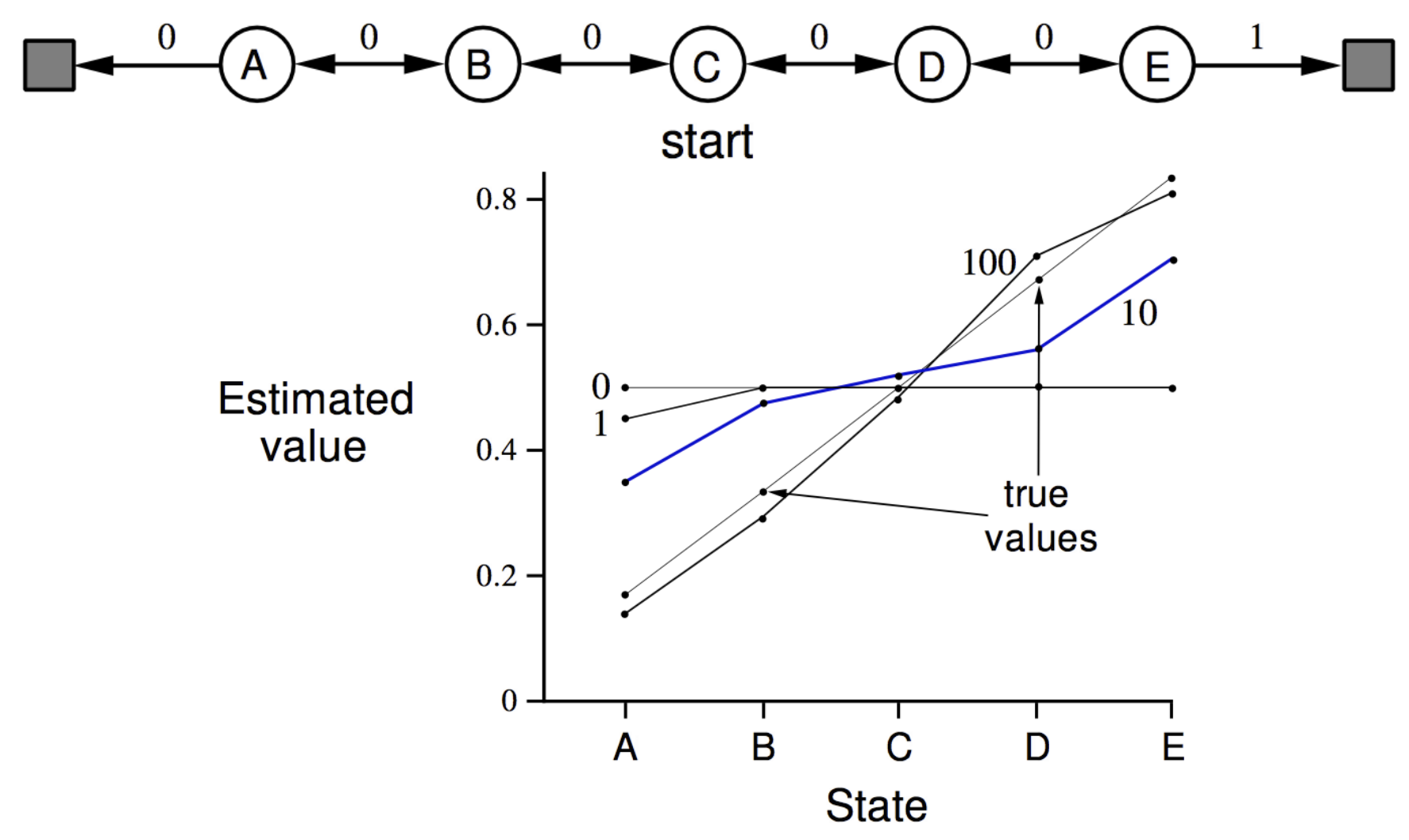
Let’s illustrate these differences with a classic example. Consider the random walk depicted above. From each state ($A$ through $E$), there are two possible actions: Left and Right. We follow a uniform random policy (equal probability of $0.5$ for each action).

• Rewards: All transitions give a reward of $0$, unless you terminate on the far right (transition from $E$), which gives a reward of $+1$.
• Termination: The episode ends if you reach the far left (reward $0$) or far right (reward $+1$).

The Question: What is the value function $v_{\pi}(s)$ for being in each of these states?

The true value of each state represents the probability of terminating on the right side. Thus, the true values form a straight diagonal line: \(V(A)=1/6, V(B)=2/6, \dots, V(E)=5/6\)

The figure above illustrates the estimated value function using the TD(0) algorithm:

• Initialization: We start with an arbitrary Value Estimate ($0.5$ for all states).
• Learning: As we run the algorithm for $1 \rightarrow 10 \rightarrow 100$ episodes, the estimated value function tilts and converges toward the true value function (the diagonal line).

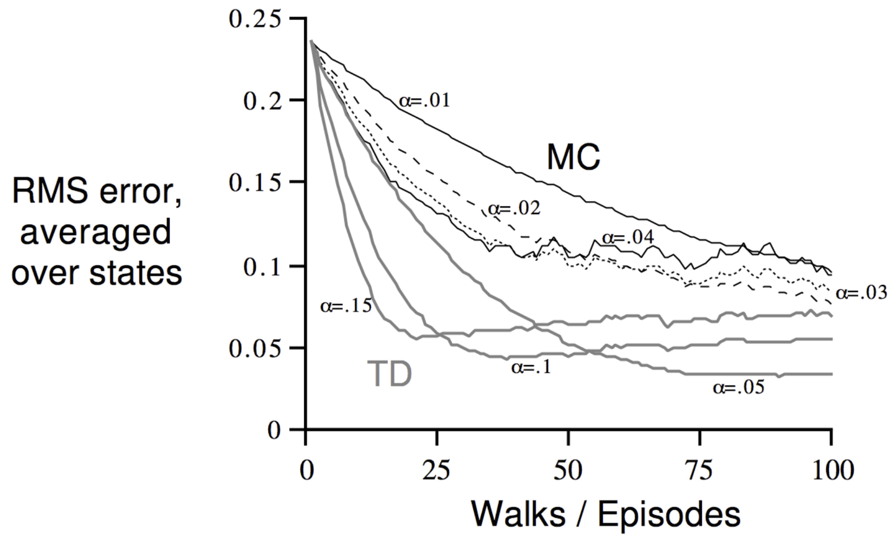
Comparing Monte Carlo vs. TD The plot above depicts the RMS error (difference between the true value function and our estimate, averaged over all states) as the number of episodes increases.

• Black Lines (Monte Carlo): Shows learning with different step sizes $\alpha$.
• Gray Lines (TD): Shows learning with different step sizes $\alpha$.

Key Takeaways:

1. TD is More Efficient: For appropriately chosen step sizes, TD (gray) consistently achieves lower error faster than Monte Carlo (black).
2. Why? (Information Propagation): TD bootstraps. If state $E$ learns it is valuable (close to the $+1$ reward), that information is passed backward to state $D$ in the very next step. MC, by contrast, must wait for a “lucky run” that starts at $A$ and successfully reaches the end to update $A$’s value. Given the randomness, “successful” runs are rare, making MC data-starved compared to TD
3. Convergence: While this plot uses fixed step sizes (which is why the error hits a “floor” rather than reaching zero), in practice, step sizes are usually decayed to achieve perfect convergence (zero error).

Batch MC & TD

• MC and TD converge: $V(s) → v_{\pi}(s)$ as experience $\rightarrow \infty$

• But what about batch solution for finite experience?

  \[\begin{aligned} s_1^1, a_1^1, r_2^1 \cdots s_{T_1}^1 \\ \vdots \\ s_1^K, a_1^K, r_2^K \cdots s_{T_K}^K \end{aligned}\]
  • e.g. Repeatedly sample episode $k \in [1,K]$
  • Apply MC or TD(0) to episode k

To illustrate the same, we take a very simple example, consider the following episodes for a two state MDP:

\[\begin{aligned} &A \ 0 \ B \ 0 \\ &B \ 1 \\ &B \ 1 \\ &B \ 1 \\ &B \ 1 \\ &B \ 1 \\ &B \ 1 \\ &B \ 0 \end{aligned}\]

Calculating Values ($V(A)$ and $V(B)$)

1. Monte Carlo (MC) Perspective MC updates based on the actual returns observed for each state.

• For State B: B was visited 8 times.
  • Returns: $1, 1, 1, 1, 1, 1, 0, 0$ (from the first episode).
  • Average: $6/8 = 0.75$.
  • $V(B) = 0.75$
• For State A: A was visited only once (in the first episode).
  • The total return for that episode was $0$.
  • $V(A) = 0$

2. TD(0) Perspective TD updates based on the Markov structure (bootstrapping).

• For State B: TD sees the same immediate outcomes as MC. $V(B)$ converges to $0.75$.
• For State A: The transition is $A \to B$ with reward $0$.
  • TD updates $V(A)$ towards $R + \gamma V(B)$.
  • Since $V(B)$ has converged to $0.75$, $V(A)$ is pulled towards $0 + 1 \cdot 0.75$.
  • $V(A) = 0.75$

Concretely:

• MC converges to solution with minimum mean-squared error

  • Best fit to the observed returns

    \[\sum_{k=1}^K\sum_{t=1}^{T_k} (G_t^k - V(s_t^k))^2\]

  • In the training data, every time we saw $A$, the return was $0$, therefore, $V(A)=0$ minimizes the error for the training set.

• TD(0) converges to solution of max likelihood Markov Model
  • Solution to the MDP $\langle \mathcal{S, A, \hat{P}, \hat{R}}, \gamma \rangle$ that best fits the data:
  \[\begin{aligned} \mathcal{P_{s,s'}^a} = \frac{1}{N(s, a)} \sum_{k=1}^K\sum_{t=1}^{T_k} \mathbf{1}(s_t^k, a_t^k, s_{t+1}^k = s, a, s') \\ \mathcal{R_{s}^a} = \frac{1}{N(s, a)} \sum_{k=1}^K\sum_{t=1}^{T_k} \mathbf{r_{t+1}^k}(s_t^k, a_t^k = s, a) \end{aligned}\]

  • The Model TD builds:

    

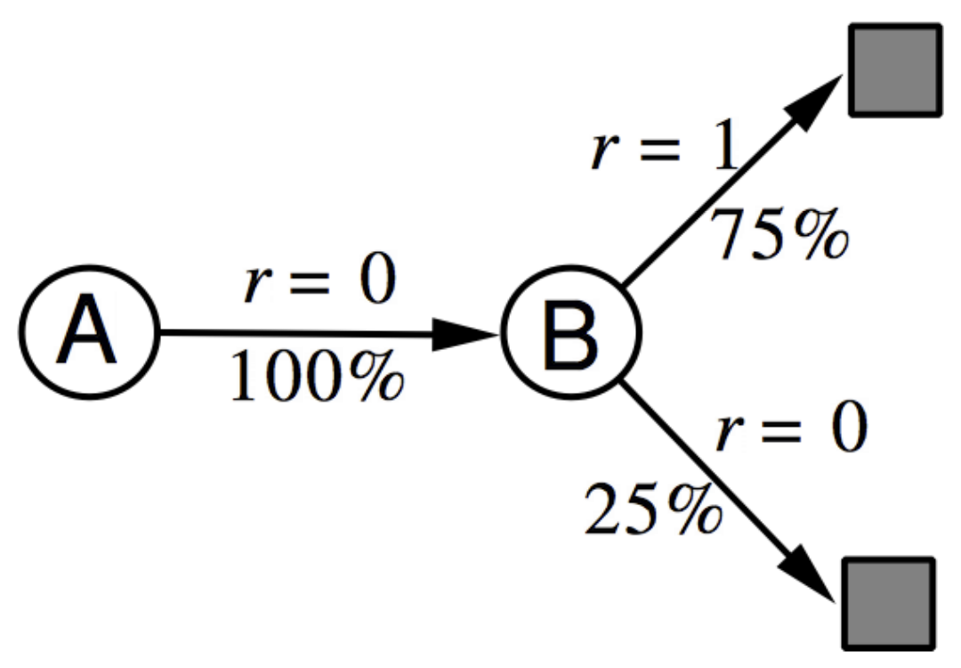
    • Transition from A: $100\%$ chance to go to B.
    • Value of B: $\approx 0.75$ (based on rewards).

  • If $A$ always goes to $B$, and $B$ is worth $0.75$, then $A$ must be worth $0.75$.

Advantages & Disadvantages (3)

TD exploits the Markov property by building implicitly an mdp structure and solving for that mdp structure. Which means that in Markov environments TD normally is more efficient because it makes use of it’s markov property than just blindly looking at complete trajectories (MC).

Whereas Monte-Carlo does not exploit the markov property, but one benefit then is if you’re in a non-markov environment (partially observed) you know you can’t just rely on the state signal. That’s when, Monte Carlo can be a better choice.

Often we have some spectrum between these where you’re maybe a little bit on Markov and then the question is how far between these (TD & MC) should you go (coming up in next section).

Summary

• Monte Carlo: Samples one complete trajectory (samples an action from the agent, then gets blow off to state by the environment (black to white node transitions) and so and so forth untill we reach a terminal state) and then you uses that to update the value function at the root of the trajectory (starting point) and we also at every intermediate state along the way to the terminal state.

  

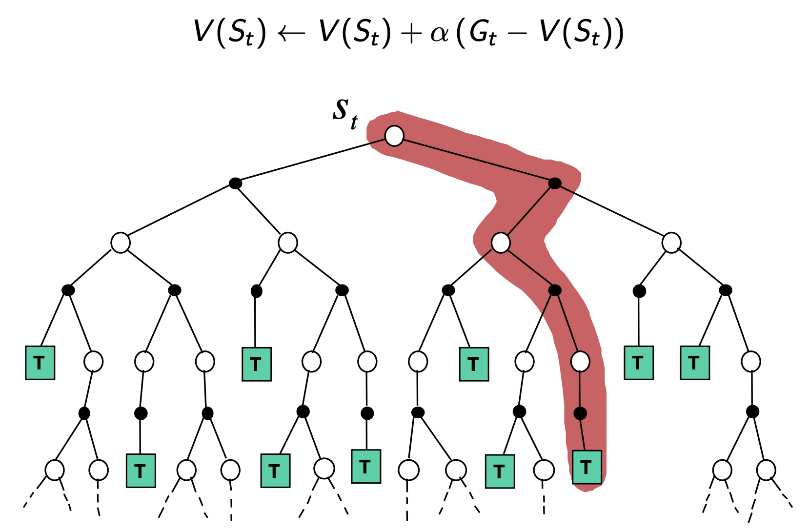
• Temporal Difference Learning: The backup is just over one step, we sample our own action, we sample the environment and then we look at the value function where we ended up. Then, we back up that value function towards the value function at the starting node.

  

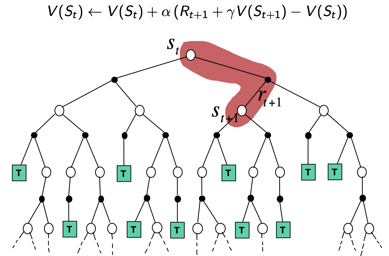
• Dynamic Programming (ref): Although we also did a one-step look ahead in DP, but n contrast to TD we didn’t sample, we knew the Dynamics and we used those Dynamics to basically compute a full expectation (as we knew the probability of where the environment would take us).

  

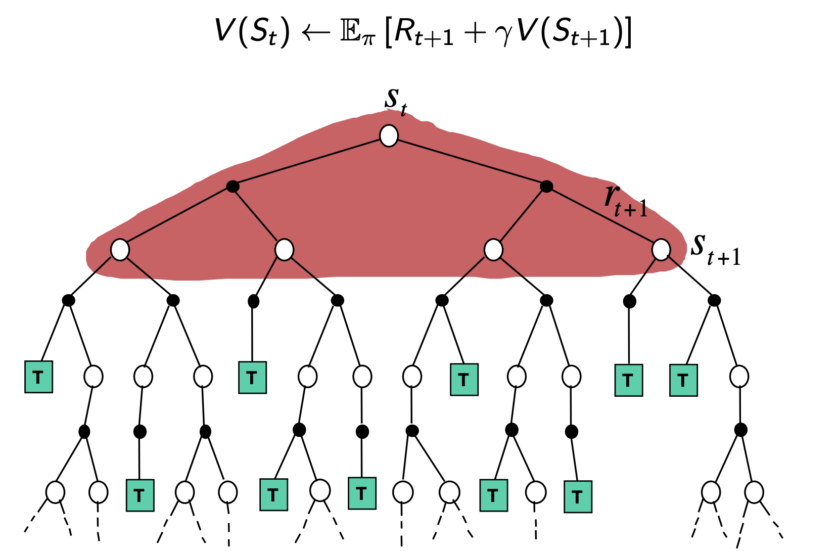
• To complete the space of possibilities, we could also do an Exhaustive look ahead of this entire tree. Essentially something which is like dynamic programming but going all the way to the end (all terminal states) and then doing a complete backup (exhaustive tree search). This intuitively, leads to an exponential blow up in the size of the update.

Unified View of RL

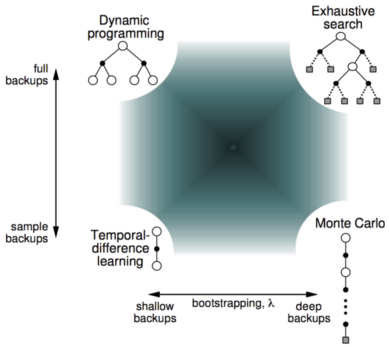
Algorithm	Bootstrapping update involves an estimate	Sampling update samples an expectation
Monte Carlo	❌	✅
Temporal Difference	✅	✅
Dynamic Programming	✅	❌

$\text{TD}(\lambda)$

N-Step TD

Instead of setting the target to immediate reward + discounted estimated value of next state, we can let the TD Target look $n$ steps into the future:

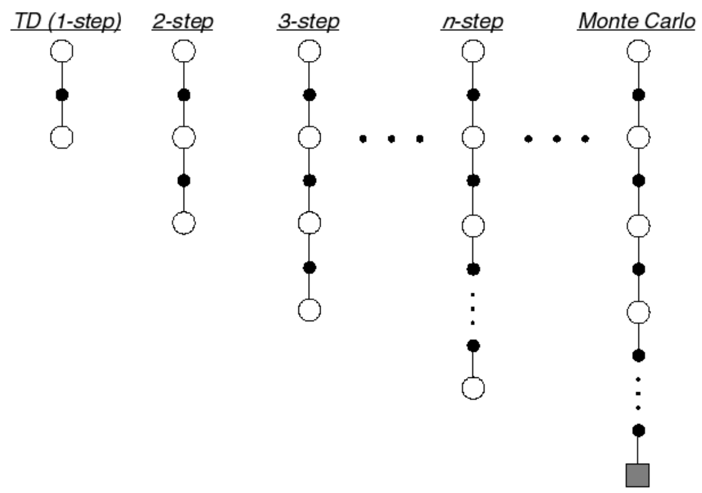
• N-step returns for $n = 1, 2, \infty$ can be written as:

  \[\begin{aligned} & n = 1 \quad \text{(TD)} \quad G_t^{(1)} = R_{t+1} + \gamma V(S_{t+1}) \\ & n = 2 \quad \text{(TD)} \quad G_t^{(2)} = R_{t+1} + \gamma R_{t+2} + \gamma^2 V(S_{t+1}) \\ & \vdots \\ & n = \infty \quad \text{(MC)} \quad G_t^{(\infty)} = R_{t+1} + \gamma R_{t+2} + \cdots + \gamma^{T-1} R_{T} \end{aligned}\]

• Or Generically, we can define N-Step return as follows:

  \[G_t^{(n)} = R_{t+1} + \gamma R_{t+2} + \cdots + \gamma^{n-1} R_{t+n} + \gamma^n V(S_{t+n})\]

• Ergo N-Step TD is then simply:

  \[V(S_t) \leftarrow V(S_t) + \alpha \left(G_t^{(n)} - V(S_t)\right)\]

Choosing the Optimal “N”

Now, the question comes down to, which “N” is the best? Is there on universal value which would apply to any problem ? To illustrate this consider the following study on the same random walk we saw before (but with more statest $\sim 21$). We track the performance in terms of RMS error and different step sizes as before, but also across different choices of n. The below summary plot shows two variations of this with online (immediate) and offline (end of episode) updates:

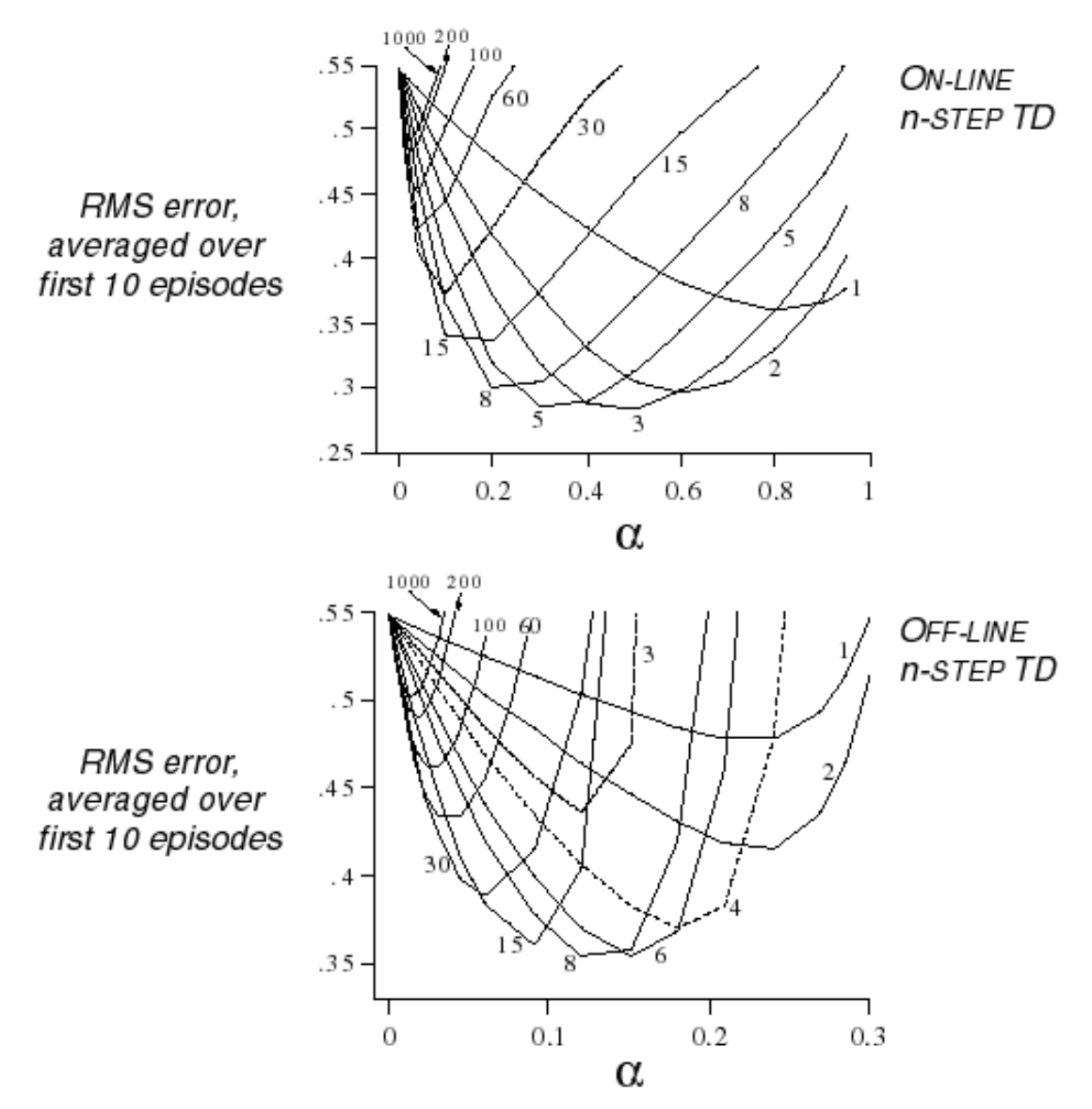
• Both show a similar character: As n approaches Infinity (approaching Monte Carlo), we start to get very high errors (the gap between the errors is exaggerated as the example was run for a shorter training time).
• In between the extremities, we get this sweet spot where if we look ahead just sort of the right number of steps in your trajectories you can propagate information backwards more efficiently (propagate information over multiple steps and hence move information more quickly across a long chain).
• However notice, that even across online & offline the optimal value of n changes! Further if we increase the size of the random walk (add more states), the optimal n would change again (favoring larger lookaheads).

Hence, we need to come up with an algorithm which gets the best of all n by efficiently considering all variations at once.

Averaging n-Step Returns

One way to consider all $n$, would be to average $n-step$ returns over different $n$:

• e.g. average the 2-step and 4-step returns \(\frac{1}{2} G^{(2)} + \frac{1}{2} G^{(4)}\)

However, can we efficiently combine information from all time-steps? Yes we can!

$\lambda$ Return

The $\lambda$ return $G_t^{\lambda}$ combines all n-step returns $G_t^{n}$ with a geometrically weighted average:

• Using weight \((1 − \lambda)\lambda^{n−1}\) for each n, giving:
• \[G_t^{\lambda} = (1 − \lambda)\sum_{n=1}^{\infty} \lambda^{n−1} G_t^{n}\]

The forward view of TD($\lambda$) is then described by:

\[V(S_t) \leftarrow V(S_t) + \alpha \left(G_t^{(\lambda)} - V(S_t)\right)\]

• These geometric weight summate to 1:

  \[\sum_{n=1}^{\infty}(1 − \lambda)\lambda^{n−1} = 1\]

• Further as can be seen in the figure:

  

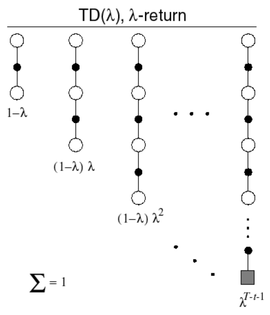
  For episodic MDPs, the largest possible $n$ gets the accumulates from $n \text{ to } \infty$. (not making sense? Think of it this way, once we reach the terminal state, from there on till infinity, we are effectively doing 0 reward transitions back to the terminal state, or in other words staying in ther terminal state!)

  

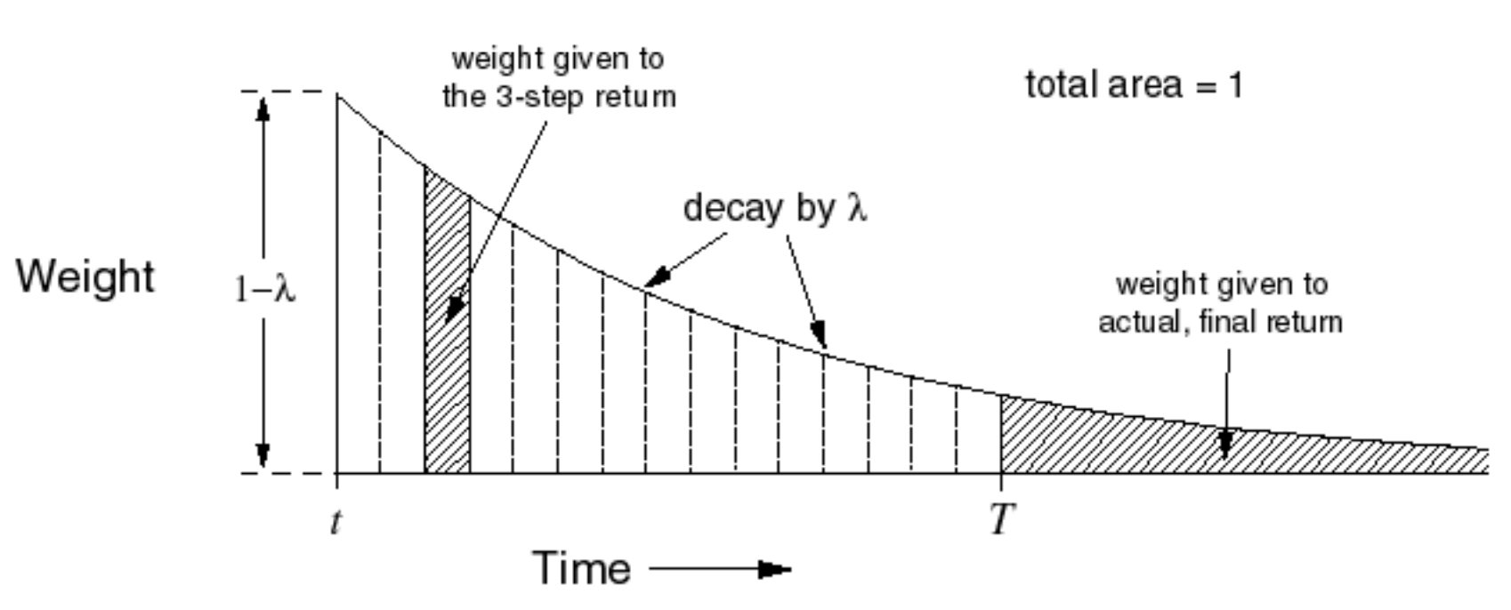
Q. Why Geometric Weighting though?

Geometric weightings are memoryless and hence effective to compute, not requiring storing or computing for each n-step return. Hence, we can effectively calcualte TD($\lambda$) in the same computational cost as TD($0$). This is may or may not be true for other weighting schemes.

It is also possible to come up with geometric weightings where the $\lambda$ varies per time step, giving us a much broader class while still having the above mentioned properties. We’ll be using this property in the upcoming lectures.

Forward View $\text{TD}(\lambda)$

Forward-view looks into the future to compute $G^{\lambda}_t$ and hence suffers from the same drawback as Monte Carlo, i.e. it can only be computed from complete episodes. But what’s nice about TD Lambda is that there exists an equivalent mechanistic view that achieves the same results as forward view $\text{TD}(\lambda)$ but without having to look into the future (without having to wait until the end of the episode). We’ll discuss that approach shortly.

Large Random Walk Example

We again look at the random walk example, but now instead plot it by varying $\lambda$.

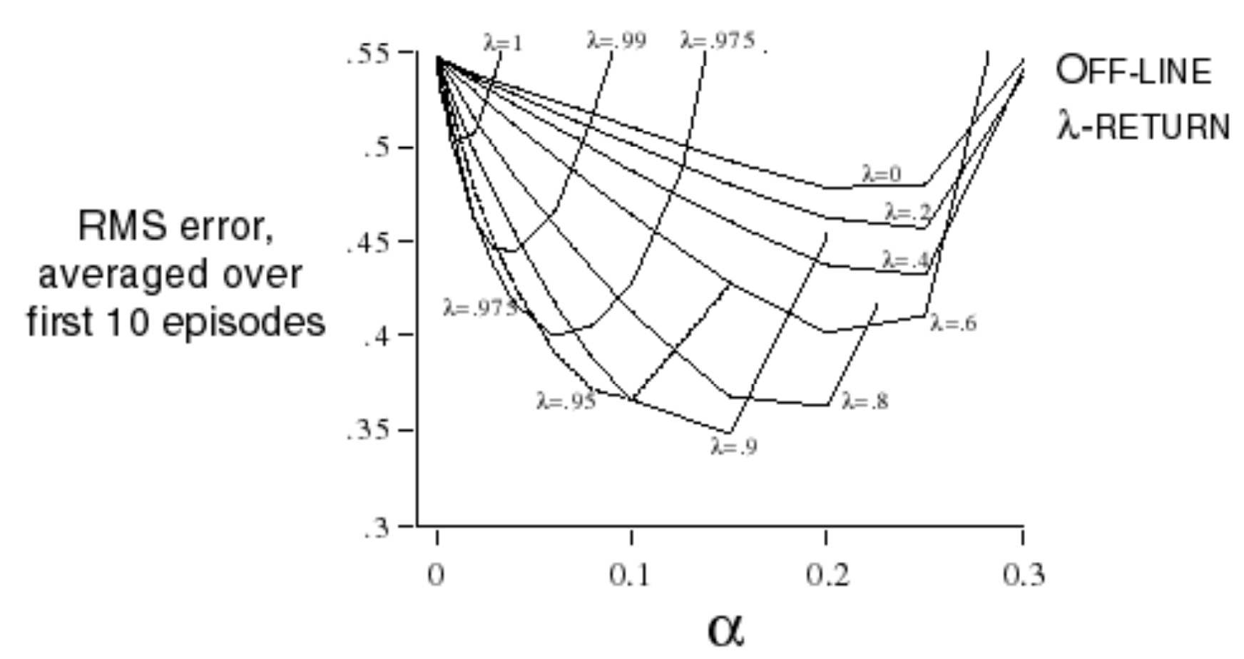
We can see that there’s a sweet spot again in $\lambda$ but it’s actually much more robust, that is it would stay the same regardless of the size of the random walk and change in the environment. In general, we often see these kind of curves where there’s a sweet spot in the $\lambda$ curve between $0$ and $1$ where we get just the right trade-off between bootstrapping and bias-variance tradeoff.

Backward View $\text{TD}(\lambda)$

The Credit Assignment Problem

Imagine you’re a rat in an experiment: you hear a bell three times, then a light comes on, and finally you get electrocuted.

Question: What caused the shock—the bell or the light?

There are two reasonable heuristics for assigning credit:

1. Frequency heuristic: Assign credit to the most frequently occurring states
   • The bell occurred more often (3 times vs 1), so blame the bell
2. Recency heuristic: Assign credit to the most recent states
   • The light was most recent before the shock, so blame the light

Eligibility traces combine both heuristics to solve the credit assignment problem.

What are Eligibility Traces?

An eligibility trace $E_t(s)$ is a short-term memory vector that tracks how “eligible” each state is for learning updates. It combines frequency and recency:

• When we visit a state, we increase its eligibility trace
• When we don’t visit a state, its eligibility trace decays exponentially

Mathematically:

\[\begin{aligned} E_0(s) &= 0 \\ E_t(s) &= \gamma\lambda E_{t-1}(s) + \mathbf{1}(S_t = s) \end{aligned}\]

where $\mathbf{1}(S_t = s)$ is 1 if we’re in state $s$ at time $t$, and 0 otherwise.

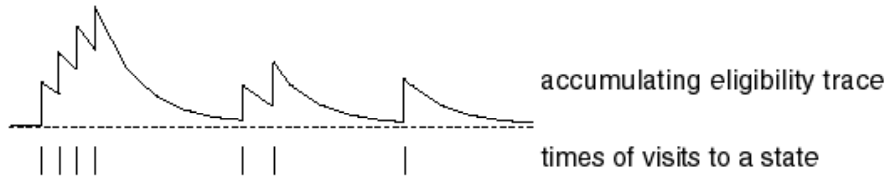
How it works:

• Each time we visit a state, we bump up its eligibility trace
• As time passes without visiting it, the trace decays
• Frequently and recently visited states have higher traces

Backward View $\text{TD}(\lambda)$ Algorithm

Instead of looking forward into the future (forward view), we can update all states by broadcasting the TD error backwards to all previously visited states, weighted by their eligibility traces.

Algorithm:

1. Keep an eligibility trace $E_t(s)$ for every state $s$

2. At each step, compute the TD error:

   \[\delta_t = R_{t+1} + \gamma V(S_{t+1}) - V(S_t)\]

3. Update the value function for ALL states (not just the current one):

   \[V(s) \leftarrow V(s) + \alpha \delta_t E_t(s)\]

4. Update eligibility traces for next step:

   \[E_{t+1}(s) = \gamma\lambda E_t(s) + \mathbf{1}(S_{t+1} = s)\]

Key insight: The TD error $\delta_t$ is broadcast backwards to all states, but the update to each state is weighted by how much credit that state deserves (its eligibility trace). States with higher eligibility get updated more.

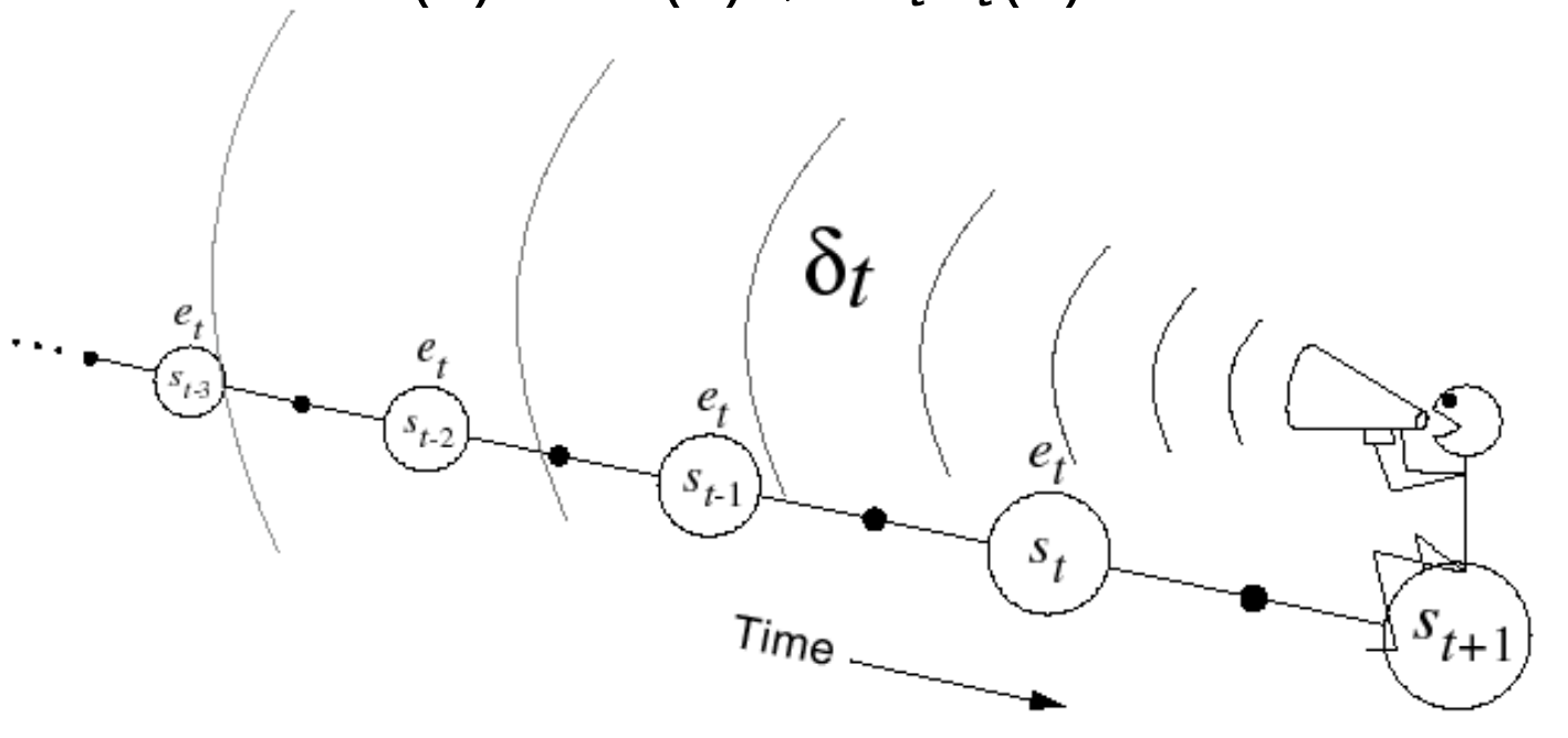
Relationship to $\text{TD}(0)$

When $\lambda = 0$:

• Eligibility traces decay immediately to zero: $E_t(s) = \gamma \cdot 0 \cdot E_{t-1}(s) + \mathbf{1}(S_t = s) = \mathbf{1}(S_t = s)$
• Only the current state has non-zero eligibility: $E_t(s) = 1$ if $s = S_t$, else $0$

• Update equation becomes:

  \[V(s) \leftarrow V(s) + \alpha \delta_t E_t(s) = V(s) + \alpha \delta_t \cdot \mathbf{1}(S_t = s)\]

• This is exactly $\text{TD}(0)$: only update the current state $S_t$

  \[V(S_t) \leftarrow V(S_t) + \alpha \delta_t\]

Relationship to Monte Carlo

When $\lambda = 1$:

• Credit is deferred until the end of the episode
• For episodic environments with offline updates (wait until episode ends, then apply all updates):

Theorem (Forward-Backward Equivalence):

The sum of offline updates is identical for forward-view and backward-view $\text{TD}(\lambda)$:

\[\sum_{t=1}^T \alpha \delta_t E_t(s) = \sum_{t=1}^T \alpha \left(G_t^\lambda - V(S_t)\right) \mathbf{1}(S_t = s)\]

In other words, summing all backward-view updates over an episode gives the same total update as summing all forward-view updates.

What this means:

• Backward view is a mechanistic implementation that achieves the same result as forward view
• You only need to look backwards (computationally efficient, no need to wait for future)
• For offline $\text{TD}(1)$, the total update equals the Monte Carlo update

Note: There exists a method, which has extended this equivalence even to online updates, where you change the value function as you go along, using a method that maintains exact equivalence.

Summary: Forward vs Backward View

Aspect	Forward View $\text{TD}(\lambda)$	Backward View $\text{TD}(\lambda)$
Update target	$G_t^\lambda$ (λ-weighted return)	$\delta_t$ (1-step TD error)
When to update	At end of episode (or after seeing future)	Immediately, every step
What to update	Current state only	All states (weighted by eligibility)
Looks at	Future returns	Past states
Equivalence	Offline updates give same total	Offline updates give same total
Efficiency	Requires seeing future	Can update online
Conceptual	Principled (what we want)	Mechanistic (how we compute)

Backward view $\text{TD}(\lambda)$ is an efficient, online-implementable algorithm that achieves the same goal as forward view $\text{TD}(\lambda)$ by cleverly broadcasting TD errors backwards using eligibility traces.

Note: Slides 44-51 were not covered explicitly in the lecture and are hence not explicitly present in these notes (I might add details later sometime in the future). If you’re interested in a mathematical derivation proving the equivalence of backward view to forward view and convergence to MC on $\lambda = 1$, checkout slides 44-51.

Misc QAs

Q. Why do we assume that the value after one step is more accurate than the value before one step? Why not reverse the dynamics and do it the other way? Would the alternative algorithm give the right answer?

Ans. It will give the wrong answer. In fact, even if you try to minimize the mean squared error of your TD error or something similar, you’ll find the wrong answer in stochastic MDPs. That’s a well-known fact—you actually get the wrong answer by doing it the other way.

The intuition is this: when you take one step, you’re always in a sense a little bit more accurate because you’ve seen one step of reality in between. That step of reality involves one step of the real reward and also one step of the real dynamics, and then you estimate your value function where you ended up. Because you’ve included one step of the real dynamics and the real reward, you are in some sense more accurate—more accurate than where you were before. If you take enough of these steps, you end up grounding yourself completely in the real dynamics and the real reward of what happened.

Whereas if you go backwards, you’re starting from a situation where you’ve already taken that step—you’re closer to your goal, you’ve already seen this real step of what happened. Now you want to move this guy towards your estimate of what happened before you saw that real step of the environment. There’s no reason to think that that estimate is actually going to be better, and often it’s going to be worse.

The key is—and this actually becomes apparent in the math if you look at the reasons these algorithms converge, like contraction mappings and so forth—it’s because you take one step of real dynamics, and that real dynamics always brings you closer to the ground truth.

Lecture 5: Model-Free Control

Notes coming out soon…

Lecture 6: Value Function Approximation

Notes coming out soon…

Lecture 7: Policy Gradient Methods

Notes coming out soon…

Lecture 8: Integrating Learning and Planning

Notes coming out soon…

Lecture 9: Exploration and Exploitation

Notes coming out soon…

Lecture 10: Case Study: RL in Classic Games

Notes coming out soon…