2 Layer NN: A Mathematical Deep Dive

Introduction

It is easy to take modern deep learning frameworks for granted. We define layers, call .backward(), and the magic happens. But treating Neural Networks as a “black box” often leads to debugging nightmares when dimensions mismatch or gradients explode.

To truly master deep learning, one must understand the engine under the hood: Matrix Calculus.

In this post, we peel back the abstraction layers by performing a rigorous mathematical deep dive into a 2-Layer Fully Connected Neural Network. We will trace the input dimensions as they transform through the forward pass, and manually derive the gradients for the backward pass. By the end of this tutorial, you won’t just know that it works—you’ll understand exactly how the numbers flow.

The Computation Graph

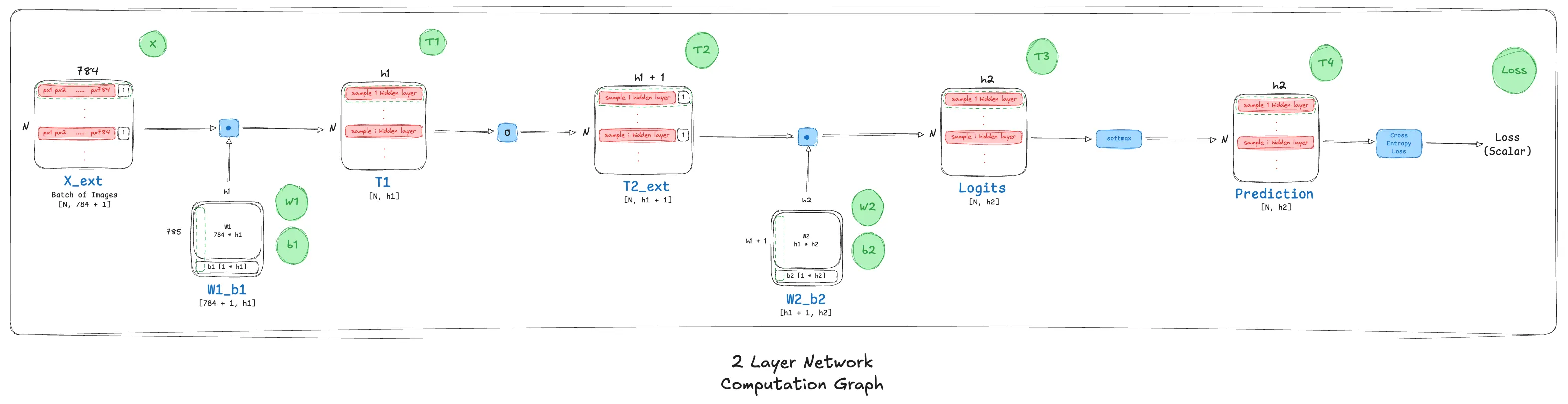
Notice that at various nodes in the graph, I have extended the layer input matrices to include a column vector of 1s, this is to accommodate bias and weight calculations together making the process a little less tedious!

Forward Pass

Input

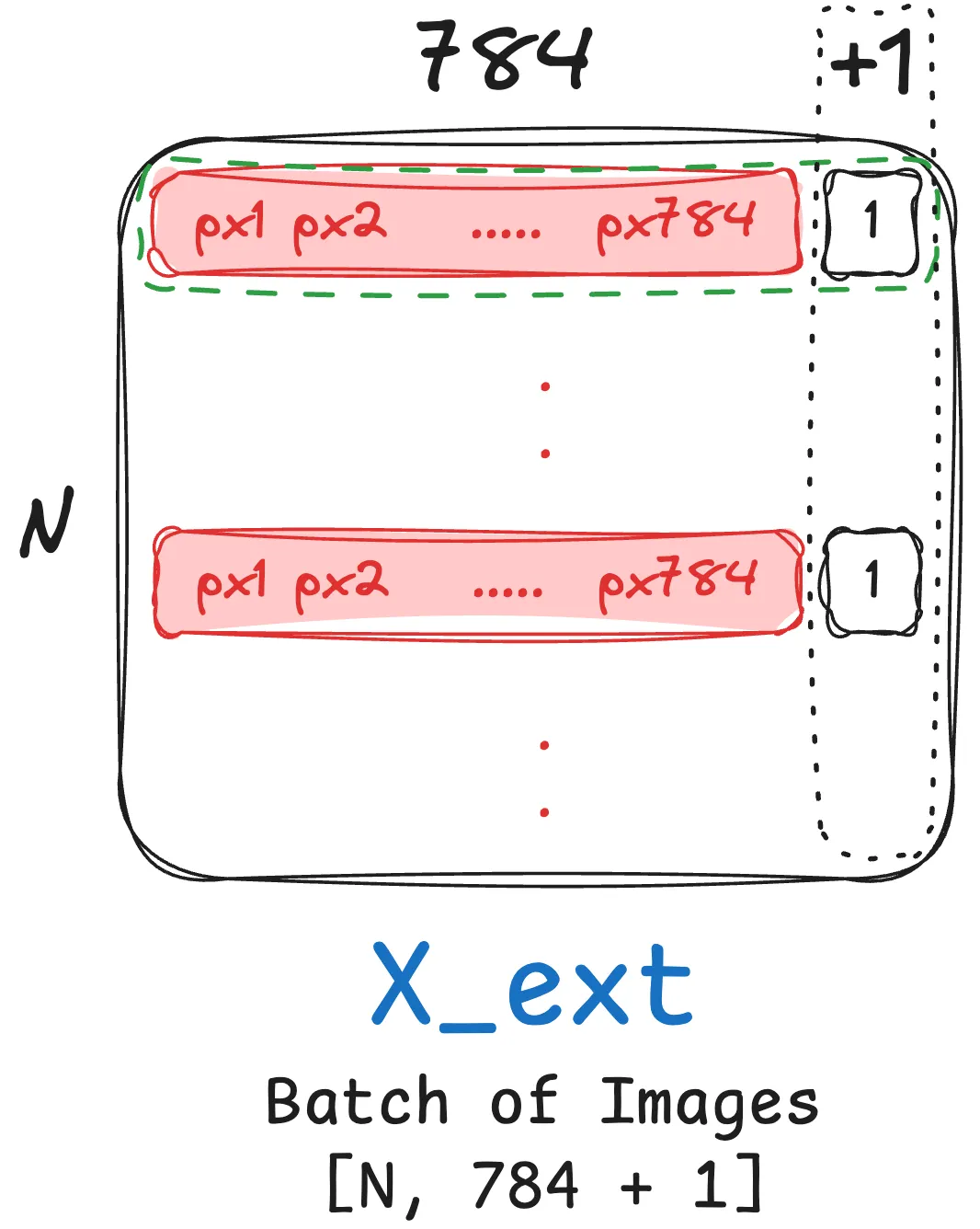
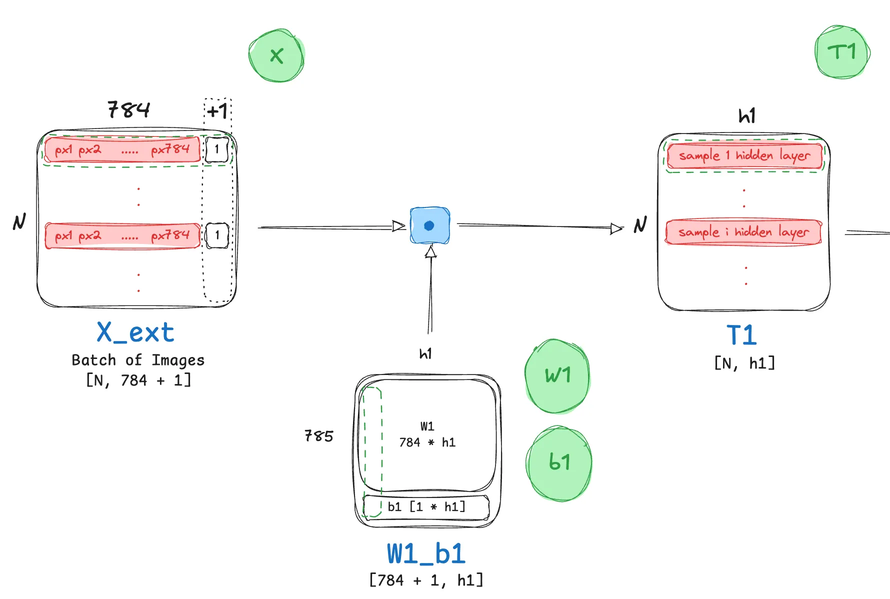
We start off with an input batch of Images:

• Each image reshaped to a row vector of size $[1, 28 \times 28] = [1, 784]$
• Assuming that we have a batch of $N$ images, the size of the input matrix now becomes $[N, 784]$.

What’s with the batch of 1s? That’s what we’re getting at in the next step!

Hidden Layer 1

Linear Transformation

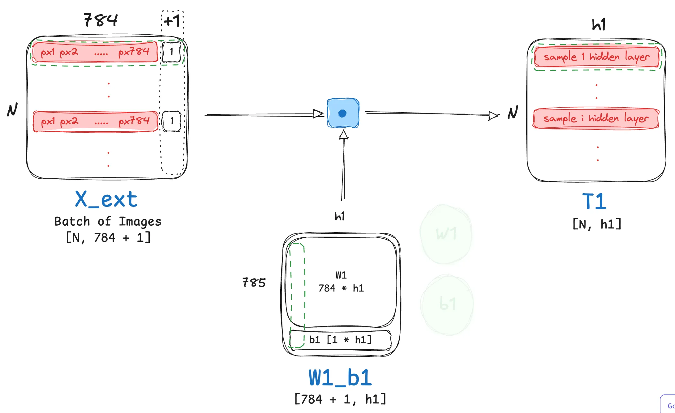
• The very first forward step in the network involves transforming each sample in the input batch from its input dimension $784$ to the representational size of the first hidden layer $h_1$. By practice, this involves a linear transformation with a weight matrix $W_1$ followed by adding a bias $b_1$. Although intuitive enough, let’s walk through the sizes of all of these matrices for our example:
  • $X \in \mathbb{R}^{N \times 784}$
  • $W_1 \in \mathbb{R}^{784 \times h_1}$
  • $b_1 \in \mathbb{R}^{1 \times h_1}$

• This leads us to the following linear transformation operation:

  $T_1 = X W_1 + b_1$

  The resulting matrix $T_1$ will have dimensions $N×h_1$, where the bias vector $b_1$ is broadcast across the N batches.

• However, this involves two operations! Looking at the expression closely we can re-write it into the following:
  • Append a column of ones to the input matrix $X$: $X_{ext} = [X \ | \ \mathbf{1}_{N \times 1}]$
  • Next, stack the bias vector $b_1$ as a new row onto the weight matrix $W_1$: $W’_1 = \begin{bmatrix} W_1 \ b_1 \end{bmatrix}$
  • The transformation then becomes a single matrix multiplication: $T_1 = X’ W’_1 = [X \ | \ \mathbf{1}] \begin{bmatrix} W_1 \ b_1 \end{bmatrix} = XW_1 + \mathbf{1}b_1$

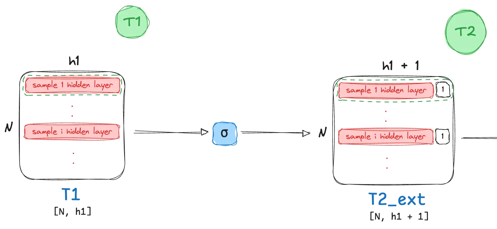
Sigmoid Activation

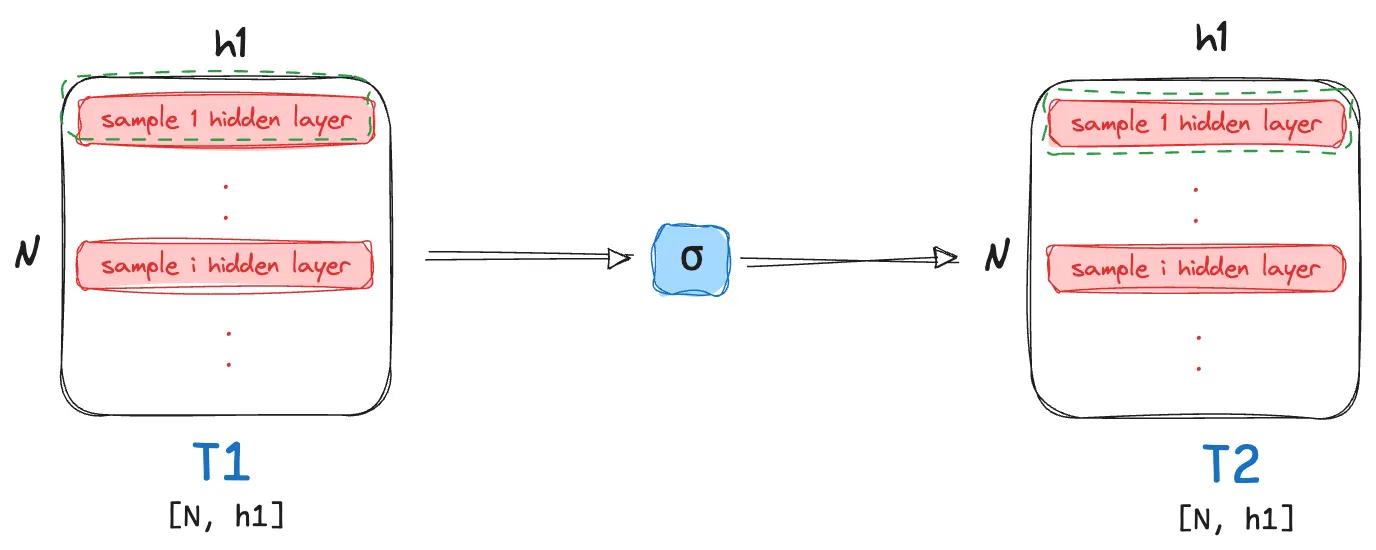
• This step involves a simple element level operation! We transform each element $t_{ij}$ of the matrix $T_1$ to $\large \tfrac{1}{1 + e^{-t_{ij}}}$.

• As this is an element level operation, the size of the resulting matrix post activation still remains the same!

  $T_2 \in \mathbb{R}^{N \times h_1}$

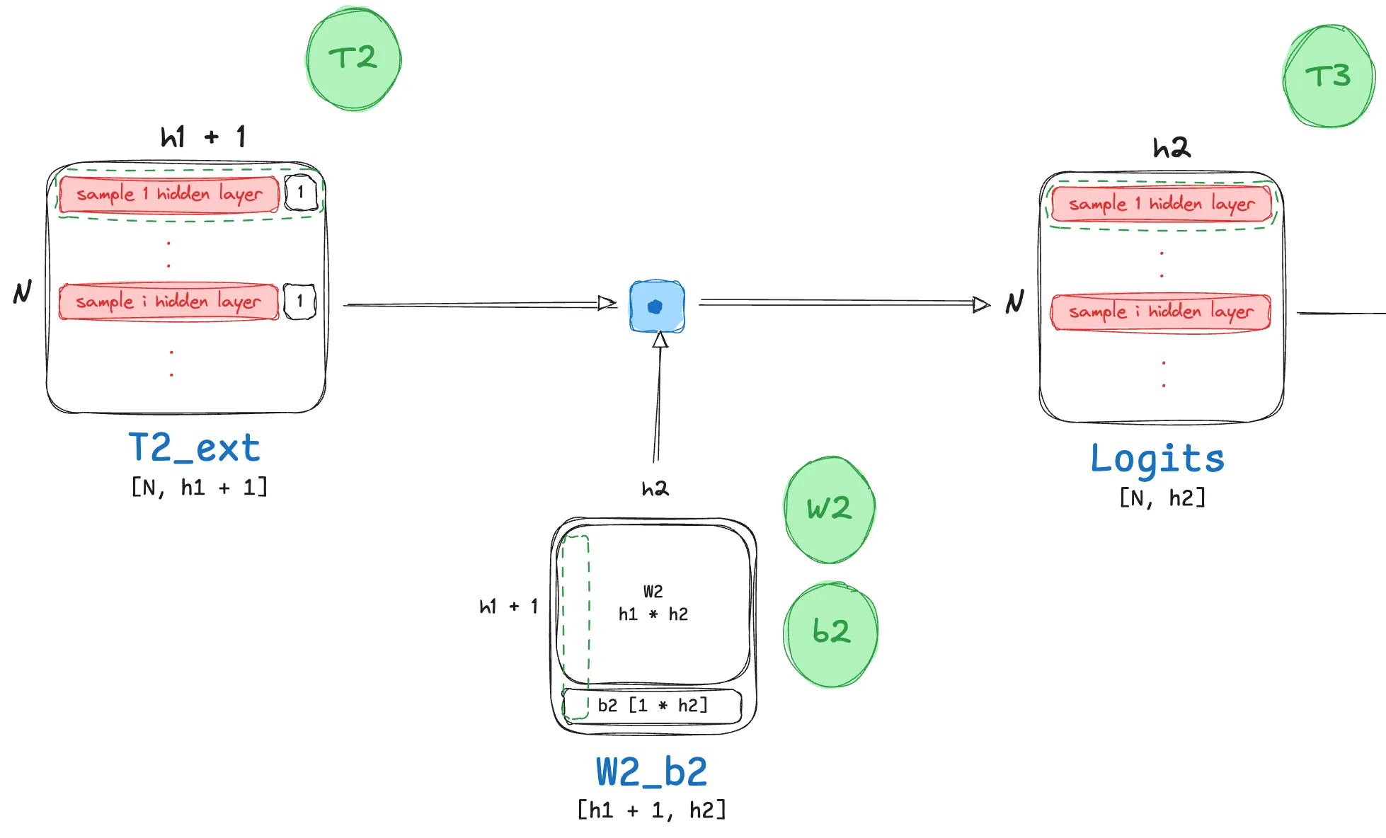
Hidden Layer 2

Linear Transformation (Logits)

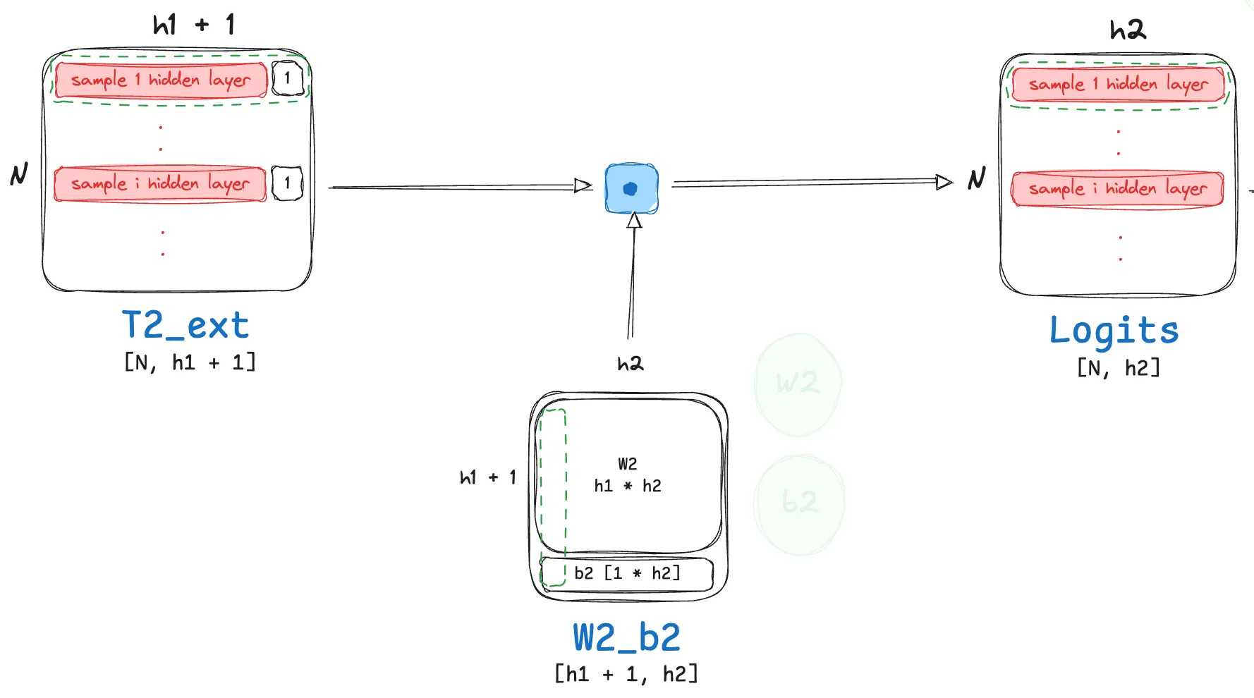
• The math here is very similar to the linear transformation step we discussed in detail for the previous hidden layer.
• As this is the final layer affecting a layer size change in the network (in case this isn’t clear, please read through till the end of the forward pass explanation!) $h_2$ below effectively will correspond to number of classes we wish to classify our input images into.
• Although intuitive enough, let’s walk through the sizes of all matrices involved in this step too:
  • $T2_{ext} \in \mathbb{R}^{N \times (h1 + 1)}$, this is the extended input matrix.
  • $W_2 \in \mathbb{R}^{h_1 \times h_2}, b_2 \in \mathbb{R}^{1 \times h_2}$
  • $W_2’ \in \mathbb{R}^{(h1 + 1) \times {h2}}$, this is the extended weight matrix.

• This leads us to the following linear transformation operation:

  \[T_3 = T2_{ext} W'_2 = [T_2 \ | \ \mathbf{1}] \begin{bmatrix} W_2 \\ b_2 \end{bmatrix} = T_2W_2 + \mathbf{1}b_2\]

  The resulting matrix $T_3$ will have dimensions $N×h_2$, where the bias vector $b_2$ is broadcast across the N batches.

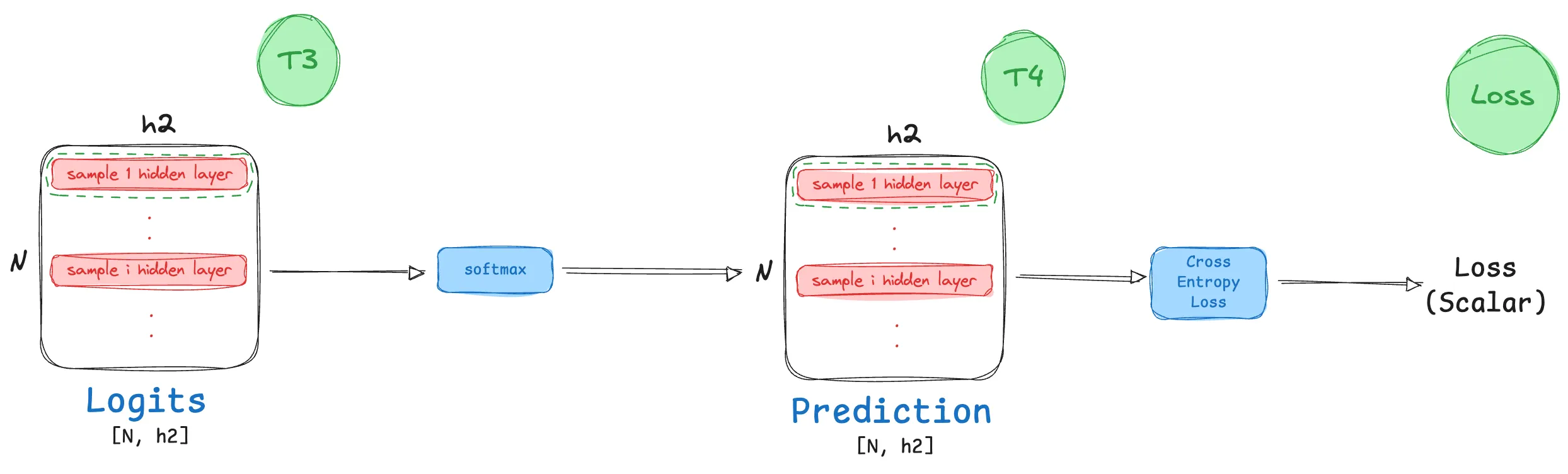
• We now have our logits (Unnormalized class output probabilities)!

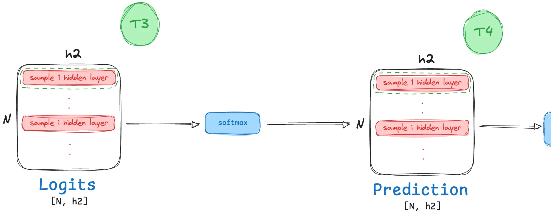
Softmax Activation (Raw > Probability Distribution)

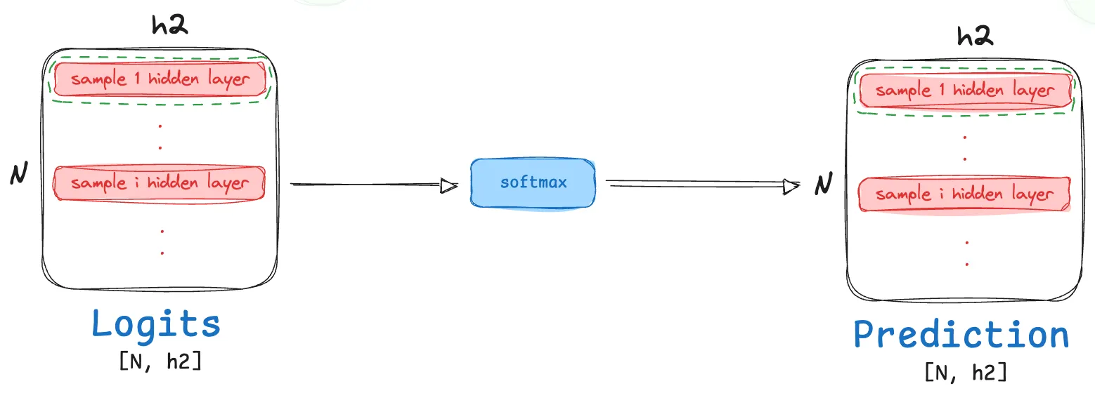
• Unlike the previous activation function, softmax is not a element level operation, however it doesn’t lead to any dimensionality change! To visually capture what this transformation looks like for a given sample layer from our hidden layer batch, consider:

  • The $ith$ row in $T_3$ (which is effectively the second layer hidden output for the $i^{th}$ image):

    \[T_{3[i,:]} = [u_0, u_1, \cdots, u_{h_2}]\]

  • Post softmax activation, this row now becomes:

    \[T_{4[i,;]} = [\tfrac{e^{u_0}}{\sum_ie^{u_i}}, \tfrac{e^{u_1}}{\sum_ie^{u_i}}, \cdots, \tfrac{e^{u_{h2}}}{\sum_ie^{u_i}}]\]
• The resulting matrix $T_4$ has dimensions same as $T_3$ i.e., $N×h_2$, with elements updated as discussed above.

Cross Entropy Loss

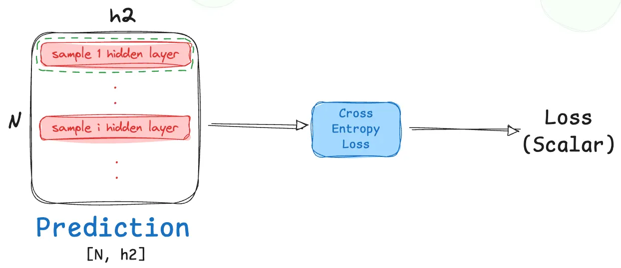
As we now have normalized probability outputs for all classes and all batches, we can now calculate loss! As we are building a multi-class classifier, the ideal loss function here would be Cross-Entropy loss. Let’s take a look at what this loss looks like for one sample in our prediction output batch.

• Consider the output probabilities for the $i^{th}$ image:

  $T_{4[i,;]} = [p_1, p_2, \cdots, p_{h_2}]$

• Now assuming that the class label (ground truth) for this image is $j$, then we can calculate the cross entropy loss for this prediction by definition as follows: \(\texttt{Loss}_i = -(\sum_ky_{[ik]}(log(T_{4[ik]}))\)

  here, $\boldsymbol{y}$ is the one-hot encoded ground truth vector (in this case it’ll be $[0\cdots 1 \cdots 0]$, where the 1 is at position $j$). Thus, the above equation simply boils down to:

  \[\texttt{Loss}_i = -y_{[ij]}(log(T_{4[ij]}))\]

• As we obtain loss from all samples / images in the batch, hence the final calculated loss is then taken as an average of these:

  \[\texttt{Loss} = -\tfrac{1}{N}\sum_i(\sum_k{y_{[ik]}}(log(T_{4[ik]}))\]

The calculated loss is a scalar entity.

Back-Propagation

Cross Entropy (Loss) → Probability Distribution (T4)

Let’s calculate first partial gradient on our journey backwards! (For obvious reasons I’ll be skipping the change in “Loss” wrt to “Loss” because that is just 1, so why even bother).

• Looking at the very last step of the forward pass, we have:

• And as we already know:

  \[\texttt{Loss} = -\tfrac{1}{N}\sum_i(\sum_k{y_{[ik]}}(log(T_{4[ik]}))\]

• Quite clearly, this scalar entity is dependent on each and every element of the $T4$ Matrix (or normalized probability classification outputs for each image). Following rules of matrix calculus, we get:

  \[\large \tfrac{\partial \texttt{Loss}}{\partial T_4} = \begin{bmatrix} \tfrac{\partial \texttt{Loss}}{T_{4[1, 1]}} & \tfrac{\partial \texttt{Loss}}{\partial T_{4[1, 2]}} & \cdots & \tfrac{\partial \texttt{Loss}}{\partial T_{4[1, h_2]}}\\ \vdots & \vdots & \ddots & \vdots \\ \tfrac{\partial \texttt{Loss}}{T_{4[N, 1]}} & \tfrac{\partial \texttt{Loss}}{\partial T_{4[N, 2]}} & \cdots & \tfrac{\partial \texttt{Loss}}{\partial T_{4[N, h_2]}}\\ \end{bmatrix} \in \mathbb{R}^{N\times h_2}\]

  (Notice that we’re using the denominator layout here, instead of numerator layout, if you’re not familiar with these terms, here’s a quick reference: wikipedia)

• Another thing to note is that:

  \[\large \tfrac{\partial \texttt{Loss}}{\partial T_{4[i, j]}} = -\tfrac{y_{[i,j]}}{N\cdot T_{4[i,j]}} = \begin{cases} -\tfrac{1}{N\cdot T_{4[i,j]}} & \small \texttt{if j = true label} \\ \large 0 & \small \texttt{else}\end{cases}\]

  this is very easily derivable, so I won’t be diving into the steps here.

Probability Distribution (T4) → Logits (T3)

Moving a step back in the graph, we reach: ($T_3 \rightarrow \texttt{softmax} \rightarrow T_4$):

• By chain rule, we can calculate:

  \[\large \tfrac{\partial \texttt{Loss}}{\partial T_3} = \tfrac{\partial \texttt{Loss}}{\partial T_4}\cdot\tfrac{\partial T_4}{\partial T_3}\]
• Let’s calculate the unknown part $\large \tfrac{\partial T_4}{\partial T_3}$, and this is where things start getting tricky, so we’ll walk through it nice and slow, making sense of each part.
  • Notice that unlike $\texttt{Loss}$, the entirety of $T_4$ is not dependent on the entirety of $T_3$, rather we are only concerned with the hidden layer activation mappings of individual samples (as we discussed earlier during forward pass).

  • Hence, quite unexpectedly our resulting Jacobian $\large \tfrac{\partial T_4}{\partial T_3}$ will be a stack of Jacobians of these individual sample level mappings! To make this even more clear, here’s what we saw earlier:

    \[T_{3[i,:]} = [u_0, u_1, \cdots, u_{h_2}] \rightarrow T_{4[i,;]} = [\tfrac{e^{u_0}}{\sum_ie^{u_i}}, \tfrac{e^{u_1}}{\sum_ie^{u_i}}, \cdots, \tfrac{e^{u_{h2}}}{\sum_ie^{u_i}}]\]

  • Hence, $\large \tfrac{\partial T_4}{\partial T_3}$is a stack of the following derivatives:

    \[\large \tfrac{\partial T_{4[i, :]}}{\partial T_{3[i, :]}} = \begin{bmatrix} \tfrac{\partial T_{4[i, 1]}}{\partial T_{3[i, 1]}} & \tfrac{\partial T_{4[i, 1]}}{\partial T_{3[i, 2]}} & \cdots & \tfrac{\partial T_{4[i, 1]}}{\partial T_{3[i, h_2]}}\\ \vdots & \vdots & \ddots & \vdots \\ \tfrac{\partial T_{4[i, h_2]}}{\partial T_{3[i, 1]}} & \tfrac{\partial T_{4[i, h_2]}}{\partial T_{3[i, 2]}} & \cdots & \tfrac{\partial T_{4[i, h_2]}}{\partial T_{3[i, h_2]}}\\ \end{bmatrix} \in \mathbb{R}^{h_2\times h_2}\]
    • Here, from forward pass, we know that $T_{4[i,j]} = \tfrac{e^{T_{3[i,j]}}}{\sum_ke^{T_{3[i,k]}}}$

    • This, then gives us two cases for the partial derivative’s value for each cell:

      \[\large \tfrac{\partial T_{4[i,j]}}{\partial T_{3[i,k]}} = \small \begin{cases}T_{4[i,j]}(1 - T_{4[i,j]}) & \texttt{if, j==k} \\ -T_{4[i,j]}(T_{4[i,k]}) & \texttt{if, }j\neq k\end{cases}\]

      (the derivation for this is left as an exercise for the reader!).

• Hence, knowing that $T_3 \rightarrow T_4$ is a sample / image level operation, we can then combine our calculated derivatives and write (for each sample):

  \[\large \tfrac{\partial \texttt{Loss}}{\partial T_{3[i,:]}} = \tfrac{\partial \texttt{Loss}}{\partial T_{4[i,:]}}\cdot\tfrac{\partial T_{4[i,:]}}{\partial T_{3[i,:]}}\]

  ($\large \tfrac{\partial \texttt{Loss}}{\partial T_{4[i,:]}}$, is just the $i^{th}$ row of the jacobian we earlier calculated).

  Dimension wise, then we can see this as: \(\mathbb{R}^{1\times h_2} \times \mathbb{R}^{h_2\times h_2} \rightarrow \mathbb{R}^{1\times h_2}\)

  Hence, \(\large \tfrac{\partial \texttt{Loss}}{\partial T_{3[i,:]}} \in \mathbb{R}^{1\times h_2} \small \implies \large \tfrac{\partial \texttt{Loss}}{\partial T_{3}} \in \mathbb{R}^{N\times h_2}\)

  (Hence, the gradient / jacobian dimensions match the node size! Phew!)

Cross Entropy (Loss) → Logits (T3) (Direct Jump, Simplification!)

That was quite a lot of math, could we have simplified it? It turns out yes! We will now derive a very famous result, which helps us directly calculate $\large \tfrac{\partial \texttt{Loss}}{\partial T_3}$!

• We have, for the $i^{th}$ sample / image:

  \(\large \tfrac{\partial \texttt{Loss}}{\partial T_{3[i,:]}} = \tfrac{\partial \texttt{Loss}}{\partial T_{4[i,:]}}\cdot\tfrac{\partial T_{4[i,:]}}{\partial T_{3[i,:]}}\), or at a cell level:

  \[\large \tfrac{\partial \texttt{Loss}}{\partial T_{3[i,k]}} = \sum_{j=1}^{h_2}\tfrac{\partial \texttt{Loss}}{\partial T_{4[i,j]}}\cdot\tfrac{\partial T_{4[i,j]}}{\partial T_{3[i,k]}}\]

  (to imagine this, think how each element in a row $\large \tfrac{\partial \texttt{Loss}}{\partial T_{3[i,:]}}$ results from matrix multiplication between the two gradients / jacobians $\tfrac{\partial \texttt{Loss}}{\partial T_{4[i,:]}}\cdot\tfrac{\partial T_{4[i,:]}}{\partial T_{3[i,:]}}$!)

• Plugging in the known derivative cases from earlier, we get:

  \[\tfrac{\partial \texttt{Loss}}{\partial T_{4[i,j]}}\cdot\tfrac{\partial T_{4[i,j]}}{\partial T_{3[i,k]}} = \small \begin{cases}-\tfrac{y_{[i,j]}}{N\cdot T_{4[i,j]}} \cdot T_{4[i,j]}(1 - T_{4[i,j]}) = -\tfrac{y_{[i,j]}}{N} \cdot (1 - T_{4[i,j]}) & \texttt{if, j==k} \\ \tfrac{y_{[i,j]}}{N\cdot T_{4[i,j]}} T_{4[i,j]}(T_{4[i,k]}) = \tfrac{y_{[i,j]}}{N} \cdot T_{4[i,k]} & \texttt{if, }j\neq k\end{cases}\]

• Great, now let’s try calculating $\large \tfrac{\partial \texttt{Loss}}{\partial T_{3[i,k]}}$ again by substituting case specific values:

  \[\large \tfrac{\partial \texttt{Loss}}{\partial T_{3[i,k]}} = \normalsize \underbrace{-\tfrac{y_{[i,k]}}{N} \cdot (1 - T_{4[i,k]})}_{j = k} + \underbrace{\sum_{j=1}^{h_2, j\neq k}\tfrac{y_{[i,j]}}{N} \cdot T_{4[i,k]}}_{j \neq k}\]

  • Looking at the term on extreme right (remember that $y$ is simply a one-hot vector, so it sums up to 1):

    \[\sum_{j=1}^{h_2, j\neq k}\tfrac{y_{[i,j]}}{N} \cdot T_{4[i,k]} = \tfrac{T_{4[i,k]}}{N}\sum_{j=1}^{h_2, j\neq k}y_{[i,j]} = \tfrac{T_{4[i,k]}}{N}(1 - y_{[i,k]})\]

  • We get:

    \[\large \tfrac{\partial \texttt{Loss}}{\partial T_{3[i,k]}} = \normalsize \underbrace{-\tfrac{y_{[i,k]}}{N} \cdot (1 - T_{4[i,k]})}_{j = k} + \underbrace{\tfrac{T_{4[i,k]}}{N}(1 - y_{[i,k]})}_{j \neq k} = \large \tfrac{T_{4[i,j]} - y_{[i,j]}}{N}\]

  (In simple terms, prediction probabilities subtracted by true probabilities averaged by batch size for each class in each sample)

Or re-writing in a more approachable manner, here’s what we just derived!

\[\large \tfrac{\partial \texttt{Loss}}{\partial T_3} = \begin{bmatrix} \tfrac{T_{4[1,1]} - y_{[1,1]}}{N} & \tfrac{T_{4[1,2]} - y_{[1,2]}}{N}& \cdots & \tfrac{T_{4[1,h_2]} - y_{[1,h_2]}}{N}\\ \vdots & \vdots & \ddots & \vdots \\ \tfrac{T_{4[N,1]} - y_{[N,1]}}{N} & \tfrac{T_{4[N,2]} - y_{[N,2]}}{N}& \cdots & \tfrac{T_{4[N,h_2]} - y_{[N,h_2]}}{N}\\ \end{bmatrix} \in \mathbb{R}^{N\times h_2}\]

Logits (T3) → Hidden Layer 1 (T2) and Second Layer Weights (\(W2\_b2\))

Now that we have the gradient of the Loss with respect to the logits, $\frac{\partial \text{Loss}}{\partial T_3}$, we can take another step back. The logits $T_3$, were calculated from the first hidden layer’s activated output $T_{2_{ext}}$ and the second layer’s weights \(W{2\_b2}\).

• Forward Pass Recall: Remember that \(T_3 = T_{2_{ext}} \cdot W{2\_b2}\). This was a simple matrix multiplication.
• Applying the Chain Rule: We need to find two gradients here:
  1. The gradient with respect to the weights, \(\frac{\partial \text{Loss}}{\partial W_{2\_b2}}\), which we need for our parameter update.
  2. The gradient with respect to the previous layer’s output, \(\frac{\partial \text{Loss}}{\partial T_2}\), which we need to continue the backpropagation.

Following the rules for matrix differentiation for the operation \(Y = XA\):

• The gradient with respect to the weights ($A$) is \(\frac{\partial L}{\partial A} = X^T \cdot \frac{\partial L}{\partial Y}\)
• The gradient with respect to the layer’s input ($X$) is \(\frac{\partial L}{\partial X} = \frac{\partial L}{\partial Y} \cdot A^T\)

Applying this to our network:

1. Gradient for Weights and Biases (\(W_{2\_b2}\))

\[\frac{\partial \text{Loss}}{\partial W2\_b2} = (T{2\_ext})^T \cdot \frac{\partial \text{Loss}}{\partial T_3}\]

Let’s check the dimensions:

• \[(T_{2\_ext})^T \in \mathbb{R}^{(h_1 + 1) \times N}\]
• \[\frac{\partial \text{Loss}}{\partial T_3} \in \mathbb{R}^{N \times h_2}\]
• Thus, the result \(\frac{\partial \text{Loss}}{\partial W2\_b2}\) has shape \([h_1 + 1, h_2]\), which perfectly matches the shape of our \(W{2\_b2}\) matrix! The all rows excepts the last row corresponds to the gradient for the weight matrix $W_2$ and the last row of this gradient matrix corresponds to the gradient for the bias $b_2$

2. Gradient for Hidden Layer Output (\(T_2\))

\[\frac{\partial \text{Loss}}{\partial T_{2_{ext}}} = \frac{\partial \text{Loss}}{\partial T_3} \cdot (W{2\_b2})^T\]

Checking the dimensions again:

• \[(W2\_b2)^T \in \mathbb{R}^{h_2 \times (h_1 + 1)}\]
• The result \(\frac{\partial \text{Loss}}{\partial T_{2_{ext}}}\) has shape \([N, h_1 + 1]\), matching \(T{2\_ext}\). The gradient has now been passed back to the previous node.

Since \(T_{2_{ext}}\) was just \(T_2\) with a column of ones concatenated, the gradient \(\frac{\partial \text{Loss}}{\partial T_2}\) is simply \(\frac{\partial \text{Loss}}{\partial T{2\_ext}}\) with the last column removed (as the gradient doesn’t flow to those constant \(1\)s).

Hidden Layer 1 Activation ($T_2$) → Hidden Layer 1 Linear ($T_1$)

This step involves back-propagating through the Sigmoid activation function.

• Forward Pass Recall: The operation was $T_2 = \text{sigmoid}(T_1)$. This is an element-wise operation.
• Applying the Chain Rule: We have the upstream gradient $\frac{\partial \text{Loss}}{\partial T_2}$ and need to find $\frac{\partial \text{Loss}}{\partial T_1}$. The chain rule for element-wise operations is a simple element-wise multiplication (a Hadamard product, denoted by $\circ$). $\frac{\partial \text{Loss}}{\partial T_1} = \frac{\partial \text{Loss}}{\partial T_2} \circ \frac{\partial T_2}{\partial T_1}$
• Derivative of Sigmoid: The derivative of the sigmoid function $\sigma(x)$ is $\sigma(x) \cdot (1 - \sigma(x))$. Since $T_2$ is the output of the sigmoid function applied to $T_1$, the derivative $\frac{\partial T_2}{\partial T_1}$ is simply $T_2 \circ (1 - T_2)$.

Combining these gives us our final gradient:

$\frac{\partial \text{Loss}}{\partial T_1} = \frac{\partial \text{Loss}}{\partial T_2} \circ (T_2 \circ (1 - T_2))$

All matrices involved here ($\frac{\partial \text{Loss}}{\partial T_1}$, $\frac{\partial \text{Loss}}{\partial T_2}$, and $T_2$) have the same dimensions, $\mathbb{R}^{N \times h_1}$, as expected for an element-wise operation.

Hidden Layer 1 Linear ($T_1$) → Input ($X$) and First Layer Weights (\(W_1\_b1\))

This is our final back-propagation step, where we calculate the gradients for the first layer’s weights and biases. The math is identical to the step for the second layer.

• Forward Pass Recall: $T_1 = X_{ext} \cdot W_{1_b1}$.
• Applying the Chain Rule: We have the upstream gradient $\frac{\partial \text{Loss}}{\partial T_1}$ and need to find $\frac{\partial \text{Loss}}{\partial W1_b1}$.

Gradient for Weights and Biases (\(W1\_b1\))

\[\frac{\partial \text{Loss}}{\partial W1\_b1} = (X_{ext})^T \cdot \frac{\partial \text{Loss}}{\partial T_1}\]

Let’s do our final dimension check:

• $(X_{ext})^T \in \mathbb{R}^{(784 + 1) \times N}$.
• $\frac{\partial \text{Loss}}{\partial T_1} \in \mathbb{R}^{N \times h_1}$.
• The result $\frac{\partial \text{Loss}}{\partial W1_b1}\in \mathbb{R}^{(784 + 1) \times h_1}$, which perfectly matches the shape of our $W{1_b1}$ matrix. As before we can easily seperate out these gradients for $W_1$ and $b_1$ if needed.

Thankyou for reading this post till the end, Hope it helped you revise or understand the concepts better (please let me know in the comments if I missed out anything :p)!